代码一:描述性统计分析和相关系数矩阵
import numpy as np
import pandas as pd

inputfile = "D:\\360MoveData\\Users\\86130\\Documents\\Tencent Files\\2268756693\\FileRecv\\data(1).csv"
data = pd.read_csv(inputfile)

#描述性统计分析
#依次计算最小值、最大值、均值、标准差
description = [data.min(),data.max(),data.mean(),data.std()]
#将结果存入数据框
description = pd.DataFrame(description,index = ['Min','Max','Mean','STD']).T
print('描述性统计结果:\n',np.round(description,2)) #保留两位小数
corr = data.corr(method = 'pearson')
print('相关系数矩阵为:\n',np.round(corr,2))
运行结果:
描述性统计结果:
             Min         Max        Mean         STD
x1   3831732.00  7599295.00  5579519.95  1262194.72
x2       181.54     2110.78      765.04      595.70
x3       448.19     6882.85     2370.83     1919.17
x4      7571.00    42049.14    19644.69    10203.02
x5      6212.70    33156.83    15870.95     8199.77
x6   6370241.00  8323096.00  7350513.60   621341.85
x7       525.71     4454.55     1712.24     1184.71
x8       985.31    15420.14     5705.80     4478.40
x9        60.62      228.46      129.49       50.51
x10       65.66      852.56      340.22      251.58
x11       97.50      120.00      103.31        5.51
x12        1.03        1.91        1.42        0.25
x13     5321.00    41972.00    17273.80    11109.19
y         64.87     2088.14      618.08      609.25
相关系数矩阵为:
x1 x2 x3 x4 x5 x6 x7 x8 x9 x10 x11 x12 \
x1 1.00 0.95 0.95 0.97 0.97 0.99 0.95 0.97 0.98 0.98 -0.29 0.94
x2 0.95 1.00 1.00 0.99 0.99 0.92 0.99 0.99 0.98 0.98 -0.13 0.89
x3 0.95 1.00 1.00 0.99 0.99 0.92 1.00 0.99 0.98 0.99 -0.15 0.89
x4 0.97 0.99 0.99 1.00 1.00 0.95 0.99 1.00 0.99 1.00 -0.19 0.91
x5 0.97 0.99 0.99 1.00 1.00 0.95 0.99 1.00 0.99 1.00 -0.18 0.90
x6 0.99 0.92 0.92 0.95 0.95 1.00 0.93 0.95 0.97 0.96 -0.34 0.95
x7 0.95 0.99 1.00 0.99 0.99 0.93 1.00 0.99 0.98 0.99 -0.15 0.89
x8 0.97 0.99 0.99 1.00 1.00 0.95 0.99 1.00 0.99 1.00 -0.15 0.90
x9 0.98 0.98 0.98 0.99 0.99 0.97 0.98 0.99 1.00 0.99 -0.23 0.91
x10 0.98 0.98 0.99 1.00 1.00 0.96 0.99 1.00 0.99 1.00 -0.17 0.90
x11 -0.29 -0.13 -0.15 -0.19 -0.18 -0.34 -0.15 -0.15 -0.23 -0.17 1.00 -0.43
x12 0.94 0.89 0.89 0.91 0.90 0.95 0.89 0.90 0.91 0.90 -0.43 1.00
x13 0.96 1.00 1.00 1.00 0.99 0.94 1.00 1.00 0.99 0.99 -0.16 0.90
y 0.94 0.98 0.99 0.99 0.99 0.91 0.99 0.99 0.98 0.99 -0.12 0.87
x13 y
x1 0.96 0.94
x2 1.00 0.98
x3 1.00 0.99
x4 1.00 0.99
x5 0.99 0.99
x6 0.94 0.91
x7 1.00 0.99
x8 1.00 0.99
x9 0.99 0.98
x10 0.99 0.99
x11 -0.16 -0.12
x12 0.90 0.87
x13 1.00 0.99
y 0.99 1.00
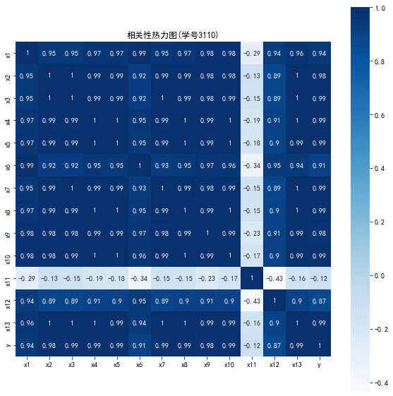
代码二:相关性热力图
import matplotlib.pyplot as plt
import seaborn as sns
plt.subplots(figsize=(10,10)) #设置画面大小
sns.heatmap(corr,annot=True,vmax=1,square=True,cmap="Blues")
plt.rcParams['font.sans-serif'] = ['SimHei'] # 添加这条可以让图形显示中文
plt.rcParams['axes.unicode_minus'] = False # 添加这条可以让图形显示负号
plt.title('相关性热力图(学号3110)')
plt.show()
plt.close
运行结果:
代码三:读取相关系数数据
import numpy as np
import pandas as pd
from sklearn.linear_model import Lasso

inputfile = "D:\\360MoveData\\Users\\86130\\Documents\\Tencent Files\\2268756693\\FileRecv\\data(1).csv"
data = pd.read_csv(inputfile) #读取数据
lasso = Lasso(1000) #调用Lasso()函数,设置λ的值为1000
lasso.fit(data.iloc[:,0:13],data['y'])
print('相关系数为:',np.round(lasso.coef_,5)) #输出结果,保留五位小数

print('相关系数非零个数为:',np.sum(lasso.coef_ !=0)) #计算相关系数非零的个数
mask = lasso.coef_ !=0 #返回一个相关系数是否为零的布尔数组
mask = np.append(mask,True) #将mask的元素补齐到14个
print('相关系数是否为零:',mask)

outputfile = "D:\\360MoveData\\Users\\86130\\Documents\\Tencent Files\\2268756693\\FileRecv\\new_reg_data.csv" #输出的数据文件
new_reg_data = data.iloc[:,mask] #返回相关系数非零的数据
new_reg_data.to_csv(outputfile) #存储数据
print('输出数据的维度为:',new_reg_data.shape) #查出输出数据的维度
运行结果:
相关系数为: [-1.8000e-04 -0.0000e+00  1.2414e-01 -1.0310e-02  6.5400e-02  1.2000e-04
  3.1741e-01  3.4900e-02 -0.0000e+00  0.0000e+00  0.0000e+00  0.0000e+00
 -4.0300e-02]
相关系数非零个数为: 8
相关系数是否为零: [ True False  True  True  True  True  True  True False False False False
  True  True]
输出数据的维度为: (20, 9)
代码四:GM11灰色预测
import sys
sys.path.append("C:\\Users\\86130\\GM11.py")
import numpy as np
import pandas as pd
from GM11 import GM11 #引入自编的灰色预测函数

inputfile1 = "D:\\360MoveData\\Users\\86130\\Documents\\Tencent Files\\2268756693\\FileRecv\\new_reg_data.csv"
inputfile2 = "D:\\360MoveData\\Users\\86130\\Documents\\Tencent Files\\2268756693\\FileRecv\\data(1).csv"
new_reg_data = pd.read_csv(inputfile1) #读取经过属性选择后的数据
data = pd.read_csv(inputfile2) #读取总的数据
new_reg_data.index = range(1994,2014)
new_reg_data.loc[2014] = None
new_reg_data.loc[2015] = None
cols = ['x1','x3','x4','x5','x6','x7','x8','x13']
for i in cols:
    f = GM11(new_reg_data.loc[range(1994, 2014),i].values)[0]
    new_reg_data.loc[2014,i] = f(len(new_reg_data)-1) #2014年预测结果
    new_reg_data.loc[2015,i] = f(len(new_reg_data)) #2015年预测结果
    new_reg_data[i] = new_reg_data[i].round(2) #保留两位小数
outputfile = ("D:\\360MoveData\\Users\\86130\\Documents\\Tencent Files\\2268756693\\FileRecv\\new_reg_data_GM11.xls") #灰色预测后保存的路径
y = list(data['y'].values) #提取财政收入列,合并至新数据框中
y.extend([np.nan,np.nan])
new_reg_data['y'] = y
new_reg_data.to_excel(outputfile) #结果输出
print('预测结果为:\n',new_reg_data.loc[2014:2015,:]) #预测展示
运行结果:
预测结果为:
Unnamed: 0 x1 x3 x4 x5 x6 \
2014 NaN 8142148.24 7042.31 43611.84 35046.63 8505522.58
2015 NaN 8460489.28 8166.92 47792.22 38384.22 8627139.31
x7 x8 x13 y
2014 4600.40 18686.28 44506.47 NaN
2015 5214.78 21474.47 49945.88 NaN
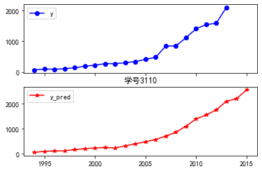
代码五:读取真实值和预测值以及绘图
import numpy as np
import pandas as pd
import matplotlib.pyplot as plt
from sklearn.svm import LinearSVR

inputfile = "D:\\360MoveData\\Users\\86130\\Documents\\Tencent Files\\2268756693\\FileRecv\\new_reg_data_GM11.xls"  # 灰色预测后保存的路径
data = pd.read_excel(inputfile)  # 读取数据
feature = ['x1', 'x3', 'x4', 'x5', 'x6', 'x7', 'x8', 'x13']  # 属性所在列

data.index = range(1994, 2016)
data_train = data.loc[range(1994, 2014)].copy()  # 取2014年前的数据建模
data_mean = data_train.mean()
data_std = data_train.std()
data_train = (data_train - data_mean)/data_std  # 数据标准化
x_train = data_train[feature].to_numpy()  # 属性数据
y_train = data_train['y'].to_numpy()  # 标签数据

linearsvr = LinearSVR()  # 调用LinearSVR()函数
linearsvr.fit(x_train,y_train)
x = ((data[feature] - data_mean[feature])/data_std[feature]).to_numpy()  # 预测,并还原结果。
data['y_pred'] = linearsvr.predict(x) * data_std['y'] + data_mean['y']
outputfile ="D:\\360MoveData\\Users\\86130\\Documents\\Tencent Files\\2268756693\\FileRecv\\new_reg_data_GM11_revenue.xls"  # SVR预测后保存的结果
data.to_excel(outputfile)

print('真实值与预测值分别为:\n',data[['y','y_pred']])

fig = data[['y','y_pred']].plot(subplots = True, style=['b-o','r-*'])  # 画出预测结果图
plt.rcParams['font.sans-serif'] = ['SimHei'] # 添加这条可以让图形显示中文
plt.title('学号3110')
plt.show()
运行结果:
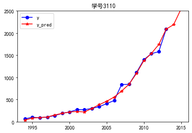
代码六:真实值和预测值重合图
import matplotlib.pyplot as plt
p = data[['y', 'y_pred']].plot(style=['b-o', 'r-*'])
p.set_ylim(0, 2500)
p.set_xlim(1993, 2016)
plt.rcParams['font.sans-serif'] = ['SimHei'] # 添加这条可以让图形显示中文
plt.title('学号3110')
plt.show()
运行结果:
代码七:读取模型的各个特征向量以及各个成分各自的方差百分比
import pandas as pd
#参数初始化
inputfile = "D:\\360MoveData\\Users\\86130\\Documents\\Tencent Files\\2268756693\\FileRecv\\principal_component(1).xls"
outputfile = "D:\\360MoveData\\Users\\86130\\Documents\\Tencent Files\\2268756693\\FileRecv\\dimention_reducted.xls"#降维后的数据

data = pd.read_excel(inputfile,header=None) #读入数据

from sklearn.decomposition import PCA

pca = PCA()
pca.fit(data)
pca.components_ #返回模型的各个特征向量
pca.explained_variance_ratio_ #返回各个成分各自的方差百分比
运行结果:
array([7.74011263e-01, 1.56949443e-01, 4.27594216e-02, 2.40659228e-02,
       1.50278048e-03, 4.10990447e-04, 2.07718405e-04, 9.24594471e-05])
代码八:运用PCA读取读取模型的各个特征向量以及各个成分各自的方差百分比
import numpy as np
from sklearn.decomposition import PCA
D = np.random.rand(10,4)
pca = PCA()
pca.fit(D)
PCA(copy=True,n_components=None,whiten=False)
pca.components_ #返回模型的各个特征向量
pca.explained_variance_ratio_ #返回各个成分各自的方差百分比
运行结果:
array([[-0.81831826,  0.08062776, -0.47242865, -0.31727837],
       [ 0.17202513,  0.44622931,  0.32588351, -0.81552848],
       [-0.08581954, -0.87700763,  0.26286504, -0.39293078],
       [-0.54166188,  0.15885902,  0.77557274,  0.28258298]])

array([0.44725817, 0.31135404, 0.1888765 , 0.05251129])

代码九:聚类中心
import numpy as np
import random
import matplotlib.pyplot as plt

def distance(point1, point2):  # 计算距离(欧几里得距离)
    return np.sqrt(np.sum((point1 - point2) ** 2))

def k_means(data, k, max_iter=10000):
    centers = {}  # 初始聚类中心
    # 初始化,随机选k个样本作为初始聚类中心。 random.sample(): 随机不重复抽取k个值
    n_data = data.shape[0]   # 样本个数
    for idx, i in enumerate(random.sample(range(n_data), k)):
        # idx取值范围[0, k-1],代表第几个聚类中心;  data[i]为随机选取的样本作为聚类中心
        centers[idx] = data[i]

    # 开始迭代
    for i in range(max_iter):  # 迭代次数
        print("开始第{}次迭代".format(i+1))
        clusters = {}    # 聚类结果,聚类中心的索引idx -> [样本集合]
        for j in range(k):  # 初始化为空列表
            clusters[j] = []

        for sample in data:  # 遍历每个样本
            distances = []  # 计算该样本到每个聚类中心的距离 (只会有k个元素)
            for c in centers:  # 遍历每个聚类中心
                # 添加该样本点到聚类中心的距离
                distances.append(distance(sample, centers[c]))
            idx = np.argmin(distances)  # 最小距离的索引
            clusters[idx].append(sample)   # 将该样本添加到第idx个聚类中心

        pre_centers = centers.copy()  # 记录之前的聚类中心点

        for c in clusters.keys():
            # 重新计算中心点(计算该聚类中心的所有样本的均值)
            centers[c] = np.mean(clusters[c], axis=0)

        is_convergent = True
        for c in centers:
            if distance(pre_centers[c], centers[c]) > 1e-8:  # 中心点是否变化
                is_convergent = False
                break
        if is_convergent == True:
            # 如果新旧聚类中心不变,则迭代停止
            break
    return centers, clusters

def predict(p_data, centers):  # 预测新样本点所在的类
    # 计算p_data 到每个聚类中心的距离,然后返回距离最小所在的聚类。
    distances = [distance(p_data, centers[c]) for c in centers]
    return np.argmin(distances)
x = np.random.randint(0,high=10,size=(200,2))
centers,clusters = k_means(x,3)
运行结果:
开始第1次迭代
开始第2次迭代
开始第3次迭代
开始第4次迭代
开始第5次迭代
开始第6次迭代
开始第7次迭代
开始第8次迭代
开始第9次迭代
开始第10次迭代
print(centers)
clusters
{0: [array([4, 9]),
  array([5, 7]),
  array([5, 5]),
  array([5, 8]),
  array([7, 6]),
  array([5, 5]),
  array([5, 9]),
  array([8, 6]),
  array([5, 9]),
  array([6, 9]),
  array([9, 7]),
  array([7, 6]),
  array([2, 9]),
  array([3, 8]),
  array([4, 9]),
  array([9, 7]),
  array([6, 6]),
  array([8, 6]),
  array([3, 7]),
  array([4, 8]),
  array([6, 5]),
  array([5, 6]),
  array([3, 8]),
  array([2, 9]),
  array([6, 8]),
  array([6, 7]),
  array([5, 7]),
  array([8, 6]),
  array([6, 9]),
  array([5, 8]),
  array([5, 8]),
  array([4, 7]),
  array([3, 8]),
  array([9, 9]),
  array([9, 7]),
  array([6, 9]),
  array([4, 6]),
  array([7, 6]),
  array([5, 7]),
  array([6, 8]),
  array([5, 8]),
  array([9, 6]),
  array([8, 9]),
  array([7, 8]),
  array([1, 9]),
  array([5, 7]),
  array([3, 9]),
  array([2, 9]),
  array([3, 7]),
  array([6, 8]),
  array([5, 9]),
  array([7, 8]),
  array([8, 6]),
  array([6, 8]),
  array([6, 7]),
  array([7, 7]),
  array([3, 7]),
  array([4, 7]),
  array([2, 8]),
  array([9, 7])],
 1: [array([5, 0]),
  array([5, 0]),
  array([9, 1]),
  array([6, 4]),
  array([6, 4]),
  array([8, 2]),
  array([7, 2]),
  array([5, 2]),
  array([6, 3]),
  array([9, 3]),
  array([7, 3]),
  array([8, 4]),
  array([8, 0]),
  array([6, 1]),
  array([5, 2]),
  array([7, 2]),
  array([8, 2]),
  array([8, 5]),
  array([7, 1]),
  array([9, 1]),
  array([7, 2]),
  array([7, 4]),
  array([6, 2]),
  array([6, 3]),
  array([8, 0]),
  array([5, 2]),
  array([5, 4]),
  array([9, 5]),
  array([6, 1]),
  array([5, 3]),
  array([4, 2]),
  array([7, 5]),
  array([4, 2]),
  array([6, 1]),
  array([8, 0]),
  array([4, 1]),
  array([7, 3]),
  array([7, 3]),
  array([7, 2]),
  array([7, 4]),
  array([7, 0]),
  array([6, 4]),
  array([8, 4]),
  array([6, 3]),
  array([7, 3]),
  array([9, 4]),
  array([8, 4]),
  array([6, 3]),
  array([9, 5]),
  array([6, 4]),
  array([7, 5]),
  array([8, 4]),
  array([9, 0]),
  array([5, 1]),
  array([4, 1]),
  array([6, 2]),
  array([8, 3])],
 2: [array([3, 4]),
  array([4, 3]),
  array([4, 5]),
  array([1, 2]),
  array([1, 8]),
  array([3, 5]),
  array([3, 2]),
  array([1, 1]),
  array([2, 2]),
  array([3, 3]),
  array([0, 5]),
  array([2, 6]),
  array([1, 7]),
  array([3, 4]),
  array([2, 2]),
  array([2, 2]),
  array([1, 6]),
  array([0, 5]),
  array([2, 6]),
  array([1, 0]),
  array([3, 2]),
  array([4, 4]),
  array([1, 5]),
  array([0, 9]),
  array([4, 5]),
  array([3, 3]),
  array([3, 1]),
  array([2, 3]),
  array([3, 6]),
  array([0, 8]),
  array([1, 4]),
  array([0, 4]),
  array([0, 0]),
  array([2, 3]),
  array([0, 8]),
  array([3, 1]),
  array([2, 1]),
  array([0, 3]),
  array([4, 5]),
  array([0, 4]),
  array([1, 3]),
  array([4, 5]),
  array([3, 0]),
  array([0, 6]),
  array([1, 5]),
  array([2, 3]),
  array([4, 3]),
  array([1, 4]),
  array([4, 5]),
  array([1, 5]),
  array([1, 3]),
  array([3, 2]),
  array([0, 4]),
  array([2, 5]),
  array([0, 4]),
  array([3, 6]),
  array([0, 9]),
  array([0, 0]),
  array([2, 5]),
  array([1, 7]),
  array([0, 9]),
  array([2, 0]),
  array([3, 5]),
  array([2, 2]),
  array([0, 5]),
  array([2, 7]),
  array([2, 1]),
  array([0, 8]),
  array([2, 7]),
  array([0, 1]),
  array([1, 2]),
  array([3, 4]),
  array([4, 4]),
  array([1, 6]),
  array([1, 1]),
  array([3, 6]),
  array([1, 2]),
  array([1, 1]),
  array([0, 3]),
  array([0, 9]),
  array([1, 2]),
  array([2, 0]),
  array([1, 6])]}

代码十:聚类中心绘图
for center in centers:
    plt.scatter(centers[center][0],centers[center][1],marker='*',s=150)

colors = ['r','b','y','m','c','g']
for c in clusters:
    for point in clusters[c]:
        plt.scatter(point[0],point[1],c = colors[c])

plt.rcParams['font.sans-serif'] = ['SimHei'] # 添加这条可以让图形显示中文
plt.title('学号3110')
运行结果:
Text(0.5, 1.0, '学号3110')

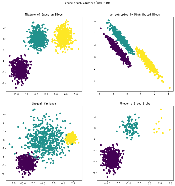
代码十一:聚类中心绘图典例
import matplotlib.pyplot as plt

fig, axs = plt.subplots(nrows=2, ncols=2, figsize=(12, 12))

axs[0, 0].scatter(X[:, 0], X[:, 1], c=y)
axs[0, 0].set_title("Mixture of Gaussian Blobs")

axs[0, 1].scatter(X_aniso[:, 0], X_aniso[:, 1], c=y)
axs[0, 1].set_title("Anisotropically Distributed Blobs")

axs[1, 0].scatter(X_varied[:, 0], X_varied[:, 1], c=y_varied)
axs[1, 0].set_title("Unequal Variance")

axs[1, 1].scatter(X_filtered[:, 0], X_filtered[:, 1], c=y_filtered)
axs[1, 1].set_title("Unevenly Sized Blobs")

plt.rcParams['axes.unicode_minus'] = False # 添加这条可以让图形显示负号
plt.rcParams['font.sans-serif'] = ['SimHei'] # 添加这条可以让图形显示中文
plt.suptitle("Ground truth clusters(学号3110)").set_y(0.95)
plt.show()
运行结果: