????前言
- ????博客主页:????睡晚不猿序程????
- ⌚首发时间:2022.7.23
- ⏰最近更新时间:2022.7.23
- ????本文由 睡晚不猿序程 原创
- ????作者是蒻蒟本蒟,如果文章里有任何错误或者表述不清,请 tt 我,万分感谢!orz
相关文章目录 :
1. 内容简介
上次我们解决了全链接网络的初始化,这次我们将会跟随着作业进一步深入,解决以下的问题:
- 完成三种优化器(SGD+momentum,RMSProp,Adam)
- 完成 Batch Normalization 以及 Layer Normalization
好的,接下来我们进入到我们的作业中去
【注】本文的代码已上传至github
2. Update rules
在之前我们一直用简单的**随机梯度下降(SGD)**作为我们的更新规则,在这一部分,我们将会构建一些最常用的更新规则,并与SGD进行对比
2.1 SGD + Momentum
这是一种带动量的更新方式,打开文件cs231n/optim.py,完成sgd_momentum,然后运行测试代码
首先我们先来看一下 SGD + Momentum 方法的代码
# Momentum update
v = mu * v - learning_rate * dx # integrate velocity
x += v # integrate position
其中 v 初始化为 0,mu 初始化为 0.9
我们可以把它理解成为,用历史的权重梯度矩阵和当前的权重梯度矩阵进行加权和,然后用此来更新 x
其中的 v 以及 mu 我们需要记录在 config 中,以在下一次更新的时候使用
我们可以很感性的理解这个梯度,我们把梯度下降想象成小球滚下山的过程,小球向下滚的时候,会它滚动的方向累计动量(也就是上面的 mu * v ),也就会朝着这个方向越滚越快( v 用 mu*v - learning_rate*dx 更新),所以这样就更有几率可以越过局部最小点,且能更快的达到收敛。
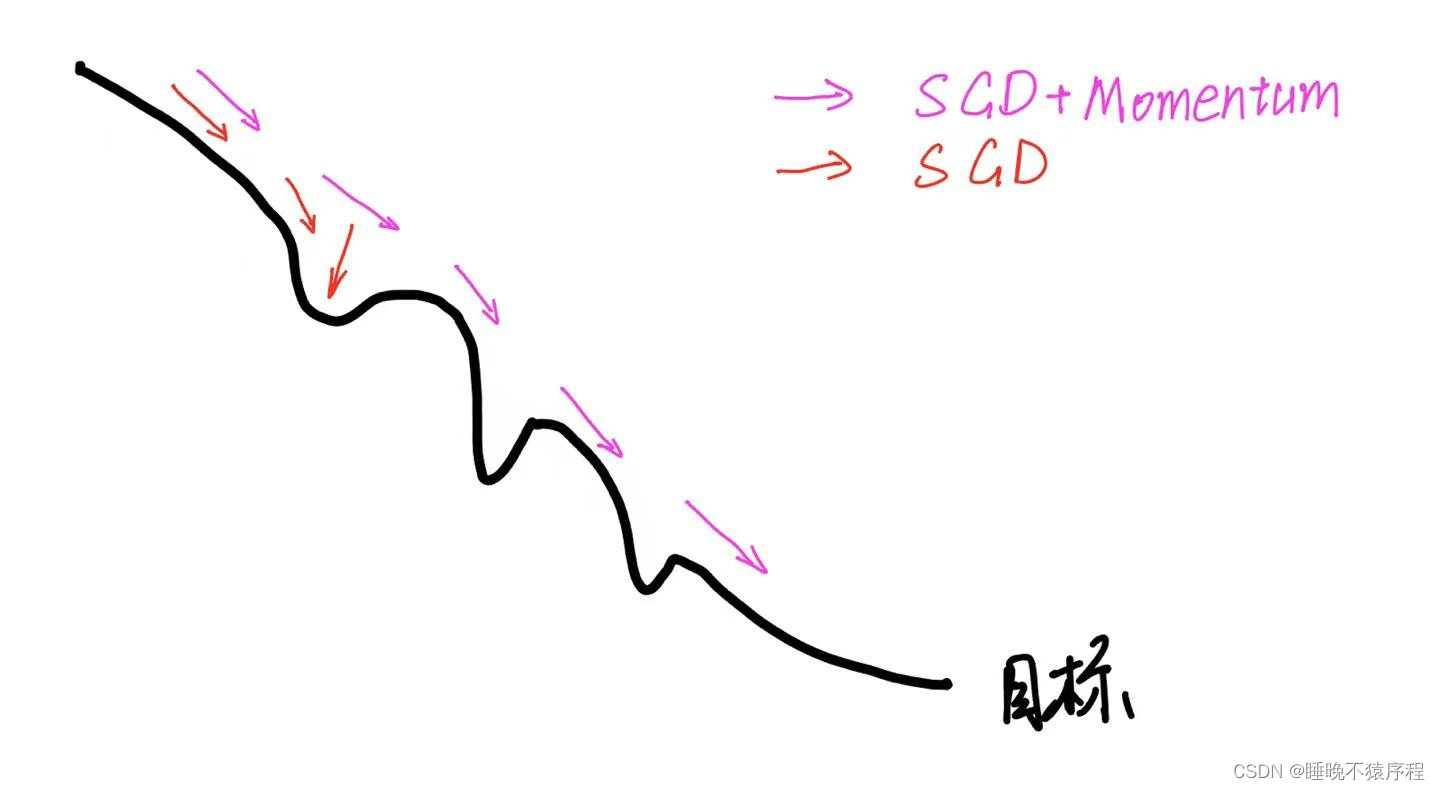
如图,如果使用简单 SGD 那么可能会被困在局部最小点中。
添加动量的好处:
- 相同的学习率下,使用动量加速的 SGD 算法可以以更大的步长进行更新
- 相同的学习率和更新时间内,动量加速可以走更多的路程,为越过那些不那么好的极小值点提供了可能性
参考资料:https://zhuanlan.zhihu.com/p/350541250
了解了SGD,接下来我们就要完成代码了:
def sgd_momentum(w, dw, config=None):
    """
    Performs stochastic gradient descent with momentum.

    config format:
    - learning_rate: Scalar learning rate.
    - momentum: Scalar between 0 and 1 giving the momentum value.
      Setting momentum = 0 reduces to sgd.
    - velocity: A numpy array of the same shape as w and dw used to store a
      moving average of the gradients.
    """
    if config is None:
        config = {}
    config.setdefault("learning_rate", 1e-2)
    config.setdefault("momentum", 0.9)
    v = config.get("velocity", np.zeros_like(w))

    next_w = None
    ###########################################################################
    # TODO: Implement the momentum update formula. Store the updated value in #
    # the next_w variable. You should also use and update the velocity v.     #
    ###########################################################################
    # *****START OF YOUR CODE (DO NOT DELETE/MODIFY THIS LINE)*****

    v=config['momentum']*v-config['learning_rate']*dw
    next_w=w+v

    # *****END OF YOUR CODE (DO NOT DELETE/MODIFY THIS LINE)*****
    ###########################################################################
    #                             END OF YOUR CODE                            #
    ###########################################################################
    config["velocity"] = v

    return next_w, config
代码解析 :
输入权重 w ,梯度 dw,存放动量以及历史梯度的字典config
v 初始化为零,照抄我们上面的公式即可
代码验证:
完成后回到 jupyter notebook 中运行,检查自己的答案是否正确

看样子是对的。
接着我们使用一个六层网络来对比 SGD 和 SGD + Momentum 二者的性能

我们会发现,SGD + Momentum 的收敛速度更快,损失更小,正确率更高
2.2 RMSProp
这是国外一个老师在某一节课堂上提出的一种优化算法
虽然 SGD+momentum 初步解决了优化过程中摆动幅度大的问题,但是可以进一步优化,并且加快收敛速度。RMSProp 对权重 W 和偏置 b 的梯度使用了微分平方加权平均数
s
d
w
=
β
s
d
w
+
(
1
−
β
)
d
W
2
s
d
b
=
β
s
d
b
+
(
1
−
β
)
d
b
2
W
=
W
−
α
d
W
s
d
w
+
ε
b
=
b
−
α
d
b
s
d
b
+
ε
s_{d w}=\beta s_{d w}+(1-\beta) d W^{2} \\ s_{d b}=\beta s_{d b}+(1-\beta) d b^{2} \\ W=W-\alpha \frac{d W}{\sqrt{s_{d w}}+\varepsilon} \\ b=b-\alpha \frac{d b}{\sqrt{s_{d b}}+\varepsilon}
sdw=βsdw+(1−β)dW2sdb=βsdb+(1−β)db2W=W−αsdw+εdWb=b−αsdb+εdb
对 dw 和 db 使用这种微分平方加权平均数 可以让其在各个维度的摆动变小,加快网络的收敛
因为,如果 dW 比较大的时候,我们需要除以其**微分平方加权平均数,**这样就可以把他降低。为了防止分母为0,使用了一个很小的数值
ϵ
ϵ
ϵ 进行平滑。
我们来看看实现的代码:
cache = config['cache']
cache = config['decay_rate']*cache + (1-config['decay_rate'])*dw**2
next_w = w-config['learning_rate']*dw/(np.sqrt(cache)+config['epsilon'])
config['cache'] = cache  # 更新cache
就是按照上面的方法进行的实现
代码解析:
config['decay_rate']就是公式中的β
\beta
β,config['learning_rate']就是公式中的α
\alpha
α- 偏置 b 被集成到了权重矩阵 W 中来方便进行运算
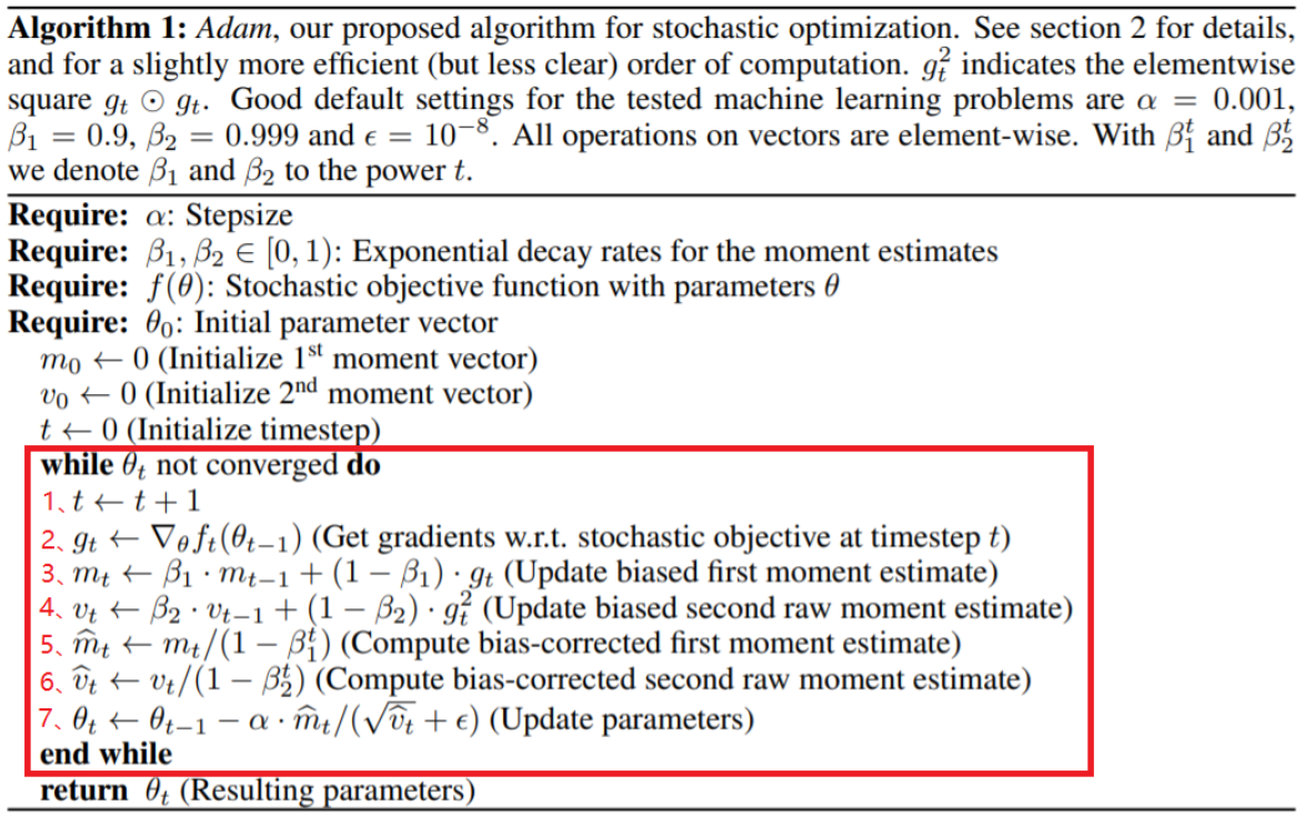
2.3 Adam
上面这两种方法各有特点,SGD+momentum 能类似物理中的动量来累计梯度,而 RMSProp 可以使得收敛速度更快同时波动的幅度变小,那么有没有可能把这两个结合起来呢?
——结合起来的答案便是,Adam
参数:
-
β
1
\beta_1
β1以及β
2
\beta_2
β2分别对应 Momentum 更新的权重和RMSProp更新的权重 -
v
d
w
v_{dw}
vdw 以及s
d
w
s_{dw}
sdw,分别对应 Momentum 的历史累计梯度以及 RMSProop 的梯度微分平方加权平均数 - 训练轮数 t,初始化为0
步骤:
- 首先将
v
d
w
v_{dw}
vdw 以及s
d
w
s_{dw}
sdw 初始化为0 - 在第 t 轮训练中,首先计算 Momentum 参数更新和 RMSProp 参数更新
- 进行偏差矫正,也就是都将更新后的
v
d
w
v_{dw}
vdw 以及s
d
w
s_{dw}
sdw 分别除以1
−
β
1
t
1-\beta_1^t
1−β1t 以及1
−
β
2
t
1-\beta_2^t
1−β2t - 将二者结合来对 W 和 b 进行更新
-
W
=
W
−
α
v
d
w
c
s
d
w
c
+
ε
W =W-\alpha \frac{v_{d w}^{c}}{\sqrt{s_{d w}^{c}}+\varepsilon}
W=W−αsdwc+εvdwc -
b
=
b
−
α
v
d
b
c
s
d
b
c
+
ε
b =b-\alpha \frac{v_{d b}^{c}}{\sqrt{s_{d b}^{c}}+\varepsilon}
b=b−αsdbc+εvdbc
-
按我自己个人的浅薄理解,就是先用 Momentum 计算出一个更细用的
m
t
m_t
mt,接着再计算出一个 RMSProp 更新所使用的
v
t
v_t
vt ,这时候把二者结合,得到更新所用的梯度。而除以
1
−
β
1
t
1-\beta_1^t
1−β1t 以及
1
−
β
2
t
1-\beta_2^t
1−β2t 是为了控制历史累计的梯度以及当前梯度的平衡。
其中,参数
β
1
\beta_1
β1我们一般取 0.9,参数我
β
1
\beta_1
β1们一般取 0.999,平滑项
ϵ
ϵ
ϵ 我们一般取
1
0
−
8
10^{-8}
10−8 ,学习率在训练的时候微调即可。
接着我们来看看代码
def adam(w, dw, config=None):
    """
    Uses the Adam update rule, which incorporates moving averages of both the
    gradient and its square and a bias correction term.

    config format:
    - learning_rate: Scalar learning rate.
    - beta1: Decay rate for moving average of first moment of gradient.
    - beta2: Decay rate for moving average of second moment of gradient.
    - epsilon: Small scalar used for smoothing to avoid dividing by zero.
    - m: Moving average of gradient.
    - v: Moving average of squared gradient.
    - t: Iteration number.
    """
    if config is None:
        config = {}
    config.setdefault("learning_rate", 1e-3)
    config.setdefault("beta1", 0.9)
    config.setdefault("beta2", 0.999)
    config.setdefault("epsilon", 1e-8)
    config.setdefault("m", np.zeros_like(w))
    config.setdefault("v", np.zeros_like(w))
    config.setdefault("t", 0)

    next_w = None
    ###########################################################################
    # TODO: Implement the Adam update formula, storing the next value of w in #
    # the next_w variable. Don't forget to update the m, v, and t variables   #
    # stored in config.                                                       #
    #                                                                         #
    # NOTE: In order to match the reference output, please modify t _before_  #
    # using it in any calculations.                                           #
    ###########################################################################
    # *****START OF YOUR CODE (DO NOT DELETE/MODIFY THIS LINE)*****
    learning_rate = config['learning_rate']
    epsilon = config['epsilon']
    t = config['t']			# 迭代轮次 t
    m = config['m']			# 历史 m
    v = config['v']			# 历史 v
    beta1 = config['beta1']	# 参数 beta1
    beta2 = config['beta2']	# 参数 beta2

    t += 1

    m = beta1*m+(1-beta1)*dw
    v = beta2*v+(1-beta2)*dw**2

    mt = m/(1-beta1**t)
    vt = v/(1-beta2**t)
    next_w = w-learning_rate*mt/(np.sqrt(vt)+epsilon)

    config['t'] = t
    config['m'] = m
    config['v'] = v
    # *****END OF YOUR CODE (DO NOT DELETE/MODIFY THIS LINE)*****
    ###########################################################################
    #                             END OF YOUR CODE                            #
    ###########################################################################

    return next_w, config
代码解析:
- 我们首先将 Adam 需要使用的参数以及历史记录读入
- 分别使用 Momentum 和 RMSProp 进行计算
- 除以 ”平衡项“ ,也就是 1-beta**t
- 进行参数更新
代码验证:
编写完成,我们运行 jupyter notebook 中的代码进行验证
RMSProp:

Adam:

我们的代码通过了验证
2.4 性能对比
我们现在拥有了四种的优化规则,也就是四种优化器,我们让他们同台竞技
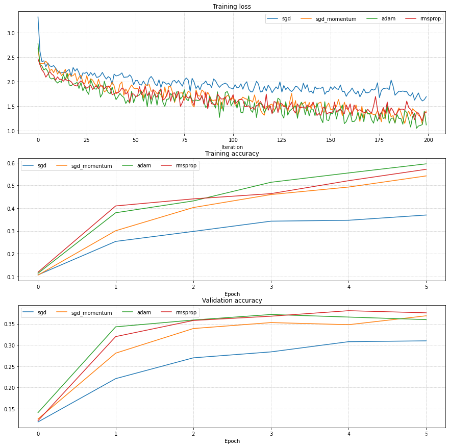
结果看起来 Adam 的效果最好
Inline Question 2
他问说,为啥使用了他写出来的这种更新规则,更新就变慢了,网络的学习也变慢了
cache += dw**2
w += - learning_rate * dw / (np.sqrt(cache) + eps)
蒻蒟的想法:我觉得是不是因为他对 dw 进行了平方操作,有的时候上游梯度非常的大,于是就限制了更新的速度,所以就更新的非常缓慢,Adam 应该不会有这个问题,因为他使用了beta1和beta2,同时一个是分子是 dw(一次方级别) 分母是 dw^2 (平方级别),不会发生指数爆炸。
更新规则我们完成了,为了训练一个良好的模型,我们还需要最后两个拼图,那就是批归一化 Batch Normalization以及Dropout
3. Batch Normalization
接下来就要进入到一个比较有难度的环节了,那就是给网络添加 BN 层,我们打开 BatchNormalization.ipynb ,开始完成此项作业
3.1 Forward Pass
在这里我们要完成 BN 层的前向传播,要完成这项作业,课程推荐我们阅读论文Sergey Ioffe and Christian Szegedy, “Batch Normalization: Accelerating Deep Network Training by ReducingInternal Covariate Shift”, ICML 2015.,我这里就简要的说一下 BN 层是个啥
我们对输入(N x D)求均值(D)方差(D),然后用均值和方差去归一化我们的整个输入,得到一个输出(N x D)
并且我们会保存一个 running_mean 和 running_var,这两个是历史均值/方差目前均值、方差的加权和,这二者只会在训练时计算,测试时直接使用这两个数据对输入数据进行归一化。
归一化层有两个可学习参数,分别为
γ
\gamma
γ 和
β
\beta
β ,这两个将会学习对归一化层进行平移
知道了这些我们直接写出代码:
def batchnorm_forward(x, gamma, beta, bn_param):
    """Forward pass for batch normalization.

    Input:
    - x: Data of shape (N, D)
    - gamma: Scale parameter of shape (D,)
    - beta: Shift paremeter of shape (D,)
    - bn_param: Dictionary with the following keys:
      - mode: 'train' or 'test'; required
      - eps: Constant for numeric stability
      - momentum: Constant for running mean / variance.
      - running_mean: Array of shape (D,) giving running mean of features
      - running_var Array of shape (D,) giving running variance of features

    Returns a tuple of:
    - out: of shape (N, D)
    - cache: A tuple of values needed in the backward pass
    """
    mode = bn_param["mode"]
    eps = bn_param.get("eps", 1e-5)
    momentum = bn_param.get("momentum", 0.9)

    N, D = x.shape
    running_mean = bn_param.get("running_mean", np.zeros(D, dtype=x.dtype))
    running_var = bn_param.get("running_var", np.zeros(D, dtype=x.dtype))

    out, cache = None, None
    if mode == "train":
        #######################################################################
        # TODO: Implement the training-time forward pass for batch norm.      #
        # Use minibatch statistics to compute the mean and variance, use      #
        # these statistics to normalize the incoming data, and scale and      #
        # shift the normalized data using gamma and beta.                     #
        #                                                                     #
        # You should store the output in the variable out. Any intermediates  #
        # that you need for the backward pass should be stored in the cache   #
        # variable.                                                           #
        #                                                                     #
        # You should also use your computed sample mean and variance together #
        # with the momentum variable to update the running mean and running   #
        # variance, storing your result in the running_mean and running_var   #
        # variables.                                                          #
        #                                                                     #
        # Note that though you should be keeping track of the running         #
        # variance, you should normalize the data based on the standard       #
        # deviation (square root of variance) instead!                        #
        # Referencing the original paper (https://arxiv.org/abs/1502.03167)   #
        # might prove to be helpful.                                          #
        #######################################################################
        # *****START OF YOUR CODE (DO NOT DELETE/MODIFY THIS LINE)*****

        sample_mean = np.mean(x, axis=0)	# 计算均值
        sample_var = np.var(x, axis=0)
        std = np.sqrt(sample_var + eps)		# 计算方差
        x_norm = (x - sample_mean) / std	# 归一化
        out = gamma * x_norm + beta			# 得到输出

        running_mean = momentum * running_mean + (1 - momentum) * sample_mean
        running_var = momentum * running_var + (1 - momentum) * sample_var

        cache = (x, x_norm, gamma, sample_mean, sample_var, eps)	# 保存反向传播需要的参数

        # *****END OF YOUR CODE (DO NOT DELETE/MODIFY THIS LINE)*****
        #######################################################################
        #                           END OF YOUR CODE                          #
        #######################################################################
    elif mode == "test":
        #######################################################################
        # TODO: Implement the test-time forward pass for batch normalization. #
        # Use the running mean and variance to normalize the incoming data,   #
        # then scale and shift the normalized data using gamma and beta.      #
        # Store the result in the out variable.                               #
        #######################################################################
        # *****START OF YOUR CODE (DO NOT DELETE/MODIFY THIS LINE)*****

        std = np.sqrt(running_var + eps)
        x_norm = (x - running_mean) / std
        out = gamma * x_norm + beta

        # *****END OF YOUR CODE (DO NOT DELETE/MODIFY THIS LINE)*****
        #######################################################################
        #                          END OF YOUR CODE                           #
        #######################################################################
    else:
        raise ValueError('Invalid forward batchnorm mode "%s"' % mode)

    # Store the updated running means back into bn_param
    bn_param["running_mean"] = running_mean
    bn_param["running_var"] = running_var

    return out, cache
代码解析:
- 训练时,计算完当前层的方差以及均值之后,记得保存到
running_var和running_mean中 - 输出为 用
γ
\gamma
γ 和β
\beta
β 对归一化后的x进行平移得到的结果。 -
γ
\gamma
γ 和β
\beta
β 是可学习参数,所以必须保存到 cache 中以便之后反向传播的时候使用。
代码验证:
写完了代码打开 jupyter notebook 进行验证
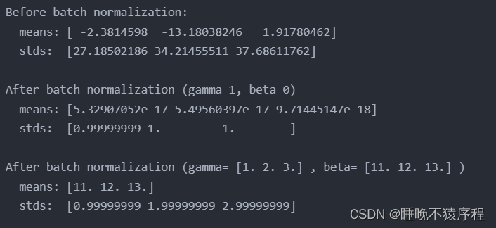
经过我们的归一化,得到了简直完美的数据
经过一次前向传播,数据的方差变为 gamma,数据的均值变为beta,符合原理
原理:
- 经过了归一化,样本的均值变为0,方差变为1
- 接下来用
o
u
t
=
x
n
o
r
m
∗
γ
+
β
out=x_{norm} * \gamma + \beta
out=xnorm∗γ+β 进行平移 - out的方差就成了 gamma,均值就变为了 beta 啦~
3.2 Backward
不知道有没有人跟我一样,一看到反向传播先头大,到底这些大神是怎么推出反向传播的公式的。这次我和大家一起慢慢推导
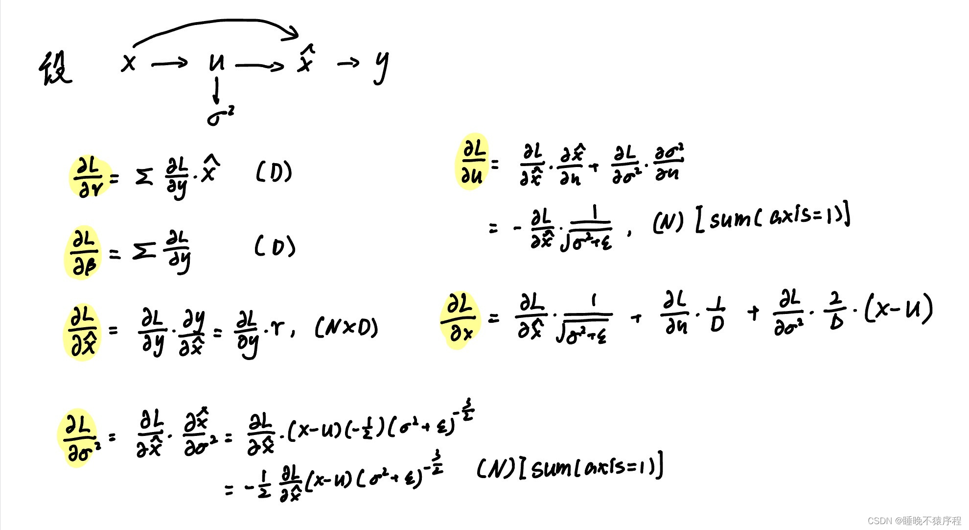
3.2.1 反向传播公式推导
首先我们先画出计算图,写出各个节点的公式备用:
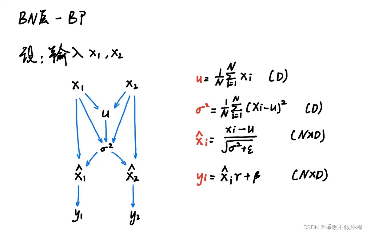
这时候我们层层向后推导:
首先是
d
γ
d\gamma
dγ 和
d
β
d\beta
dβ:
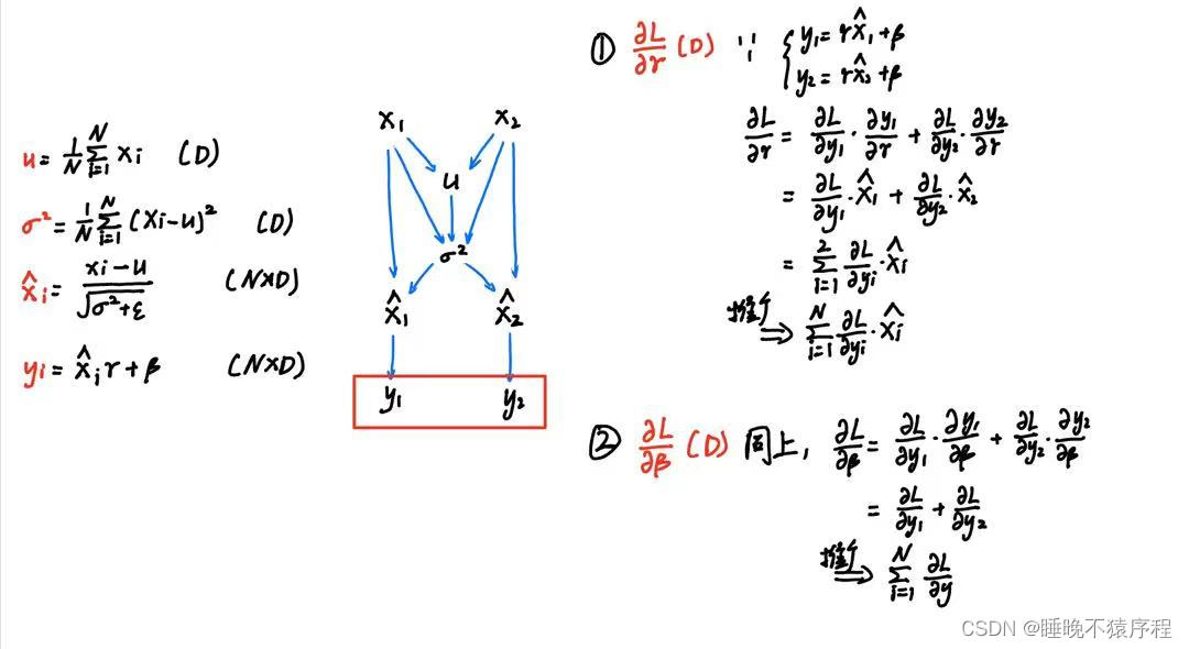
【注】利用矩阵(向量)梯度的形状和本身的形状应该是相同的来判断是很有帮助的
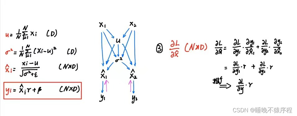
接下来是 dx_norm:
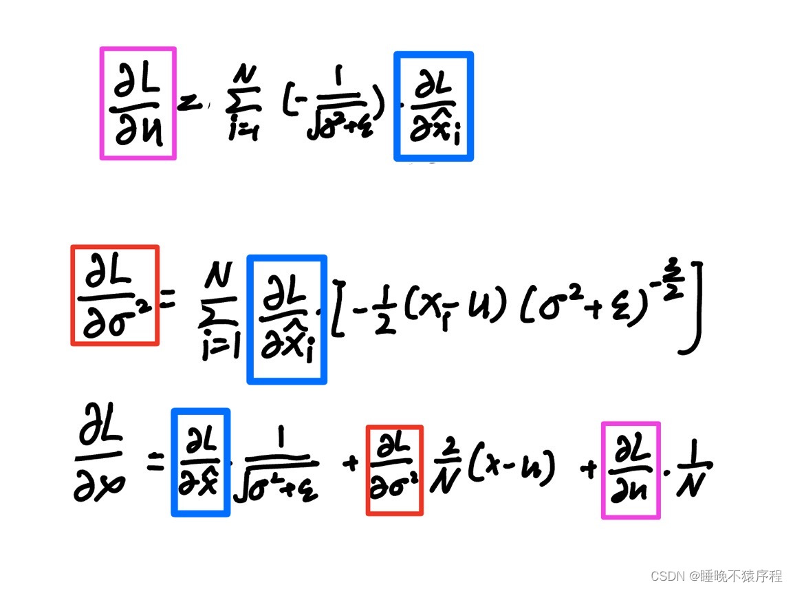
继续向前,得到 du 和 dvar:
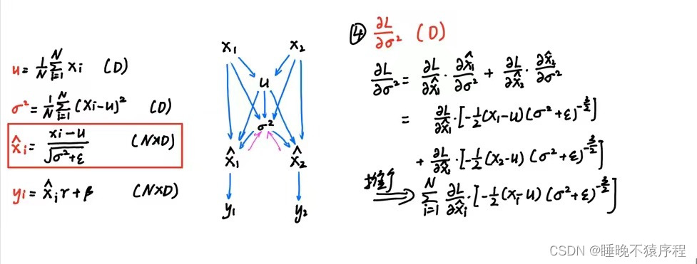
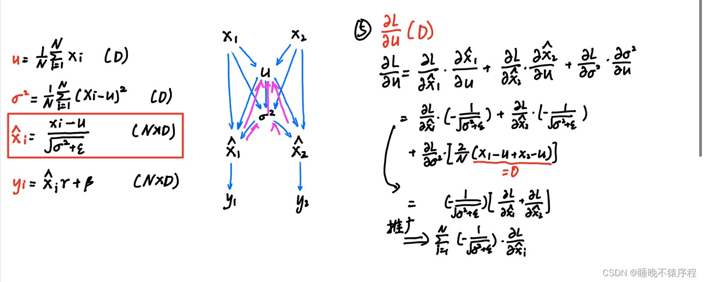
注意这里,后项是为零的,因为N个输入的和减去N乘以输入的平均数是等于零的
最后是我们的 dx 啦:
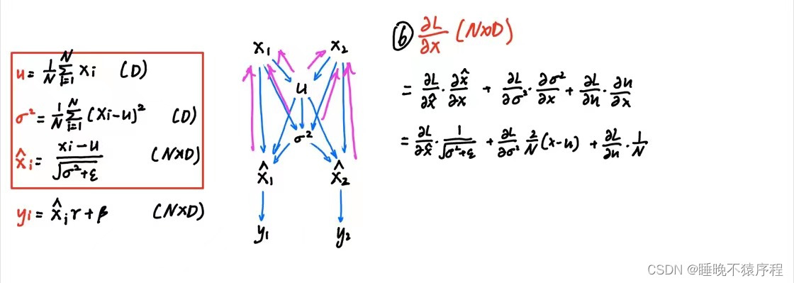
因为dx如果再用 x1 ,x2 举例的话要写好长,我直接用矩阵表示啦~
好了,接下来就按照我们所写的公式来写代码就好了:
def batchnorm_backward(dout, cache):
    """Backward pass for batch normalization.

    For this implementation, you should write out a computation graph for
    batch normalization on paper and propagate gradients backward through
    intermediate nodes.

    Inputs:
    - dout: Upstream derivatives, of shape (N, D)
    - cache: Variable of intermediates from batchnorm_forward.

    Returns a tuple of:
    - dx: Gradient with respect to inputs x, of shape (N, D)
    - dgamma: Gradient with respect to scale parameter gamma, of shape (D,)
    - dbeta: Gradient with respect to shift parameter beta, of shape (D,)
    """
    dx, dgamma, dbeta = None, None, None
    ###########################################################################
    # TODO: Implement the backward pass for batch normalization. Store the    #
    # results in the dx, dgamma, and dbeta variables.                         #
    # Referencing the original paper (https://arxiv.org/abs/1502.03167)       #
    # might prove to be helpful.                                              #
    ###########################################################################
    # *****START OF YOUR CODE (DO NOT DELETE/MODIFY THIS LINE)*****

    # (x,x_norm,gamma,sample_mean,sample_var,eps)
    x, x_norm, gamma, sample_mean, sample_var, eps = cache
    dgamma = np.sum(dout * x_norm, axis=0)  # 注意这个 *gamma 不是点乘
    dbeta = np.sum(dout, axis=0)  # 求出 dbeta
    dLdx_norm = dout * gamma
    dLdvar = np.sum(dLdx_norm * (-0.5 * (x - sample_mean) *
                                 ((sample_var + eps)**(-1.5))),
                    			 axis=0)
    dLdu = np.sum(-1 / np.sqrt(sample_var + eps) * dLdx_norm, axis=0)
    dLdx = dLdx_norm*(1/np.sqrt(sample_var+eps))+dLdvar * \
        (2/x.shape[0])*(x-sample_mean)+dLdu/x.shape[0]

    dx = dLdx

    # *****END OF YOUR CODE (DO NOT DELETE/MODIFY THIS LINE)*****
    ###########################################################################
    #                             END OF YOUR CODE                            #
    ###########################################################################

    return dx, dgamma, dbeta
代码详解:
- 注意在求 du 和 dvar 的时候,他们的形状都是(D),也就是一个D维的向量,所以我们需要对 axis = 0 进行求和
代码验证:
经过了这么复杂的计算,终于得到答案了,验证一下把!
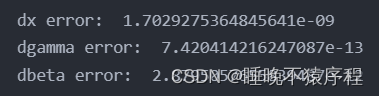
功夫不负有心人,正确了!!!/(ㄒoㄒ)/~~
【笔者写了半天写出来的一瞬间感动哭了呜呜呜】
3.3 Batch Normalization:Alternative Backward Pass
我们因为我们使用反向传播,中途计算了很多的中间变量(比如我们不需要的dvar和du)
我们可以直接从头开始,经过一系列复杂的运算,直接得出答案,这样速度更快(作者晕。。(((φ(◎ロ◎;)φ))))
说人话:就是化简,我们直接观察
发现了吗?似乎可以通过 dx_norm 来进行化简
但是,好像我搞不大明白iai,就简单的化简了一下下:
代码详解:
def batchnorm_backward_alt(dout, cache):
    """Backward pass for batch normalization.

    Inputs:
    - dout: Upstream derivatives, of shape (N, D)
    - cache: Variable of intermediates from batchnorm_forward.

    Returns a tuple of:
    - dx: Gradient with respect to inputs x, of shape (N, D)
    - dgamma: Gradient with respect to scale parameter gamma, of shape (D,)
    - dbeta: Gradient with respect to shift parameter beta, of shape (D,)
    """
    dx, dgamma, dbeta = None, None, None
    ###########################################################################
    # TODO: Implement the backward pass for batch normalization. Store the    #
    # results in the dx, dgamma, and dbeta variables.                         #
    #                                                                         #
    # After computing the gradient with respect to the centered inputs, you   #
    # should be able to compute gradients with respect to the inputs in a     #
    # single statement; our implementation fits on a single 80-character line.#
    ###########################################################################
    # *****START OF YOUR CODE (DO NOT DELETE/MODIFY THIS LINE)*****

    x, x_norm, gamma, sample_mean, sample_var, eps = cache
    N = x.shape[0]
    dbeta = np.sum(dout, axis=0)
    dgamma = np.sum(x_norm * dout, axis=0)

    std = np.sqrt(sample_var + eps)
    dLdx_norm = dout * gamma

    dLdvar = np.sum(dLdx_norm * -0.5 * (x - sample_mean) * (std**-3), axis=0)
    dLdu = np.sum(dLdx_norm * -1 / std, axis=0)

    dx = dLdx_norm / std + dLdvar * 2 / N * (x - sample_mean) + dLdu / N

    # *****END OF YOUR CODE (DO NOT DELETE/MODIFY THIS LINE)*****
    ###########################################################################
    #                             END OF YOUR CODE                            #
    ###########################################################################

    return dx, dgamma, dbeta
- 这次没有详解,就是简单的合并下
代码验证:
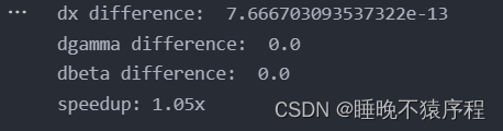
快了一点点点。。。
3.4 将 BN 层加入全连接网络中
他推荐我们,先去cs231n/layer_utils.py 添加前向传播和反向传播的代码,以让我们的实现更为容易,那么我们开工!
3.4.1 添加 Sandwich layer
打开cs231n/layer_utils.py,为了之后方便,我们构建一个affine——bn——relu 的Sandwich layer,写出他的前向传播代码
affine_bn_relu_forward:
def affine_bn_relu_forward(x,w,b,gamma,beta,bn_param):
    fc_out, fc_cache = affine_forward(x, w, b)
    bn_out, bn_cache= batchnorm_forward(fc_out,gamma,beta,bn_param)
    out,relu_cache =relu_forward(bn_out)
    cache=(fc_cache,bn_cache,relu_cache)
    return out,cache
affine_bn_relu_backward:
def affine_bn_relu_backward(dout,cache):
    fc_cache,bn_cahe,relu_cache=cache
    drelu=relu_backward(dout,relu_cache)
    dbn,dgamma,dbeta=batchnorm_backward(drelu,bn_cahe)
    dx,dw,db=affine_backward(dbn,fc_cache)
    return dx,dw,db,dgamma,dbeta
实现的代码较为简单,只需要调用我们刚刚实现的函数就可以啦
3.4.2 在 fc_net 中添加 BN 判断
在之前,我们已经实现了初始化,如果使用归一化的话,初始化将会连归一化的参数一起进行初始化
初始化函数部分的答案:
layer_dims = np.hstack((input_dim, hidden_dims, num_classes))

for i in range(self.num_layers):
W = np.random.normal(loc=0.0, scale=weight_scale, size=(layer_dims[i], layer_dims[i+1]))
b = np.zeros(layer_dims[i+1])

self.params['W' + str(i+1)] = W
self.params['b'+str(i+1)] = b

if normalization != None:
for i in range(self.num_layers-1):
gamma = np.ones(layer_dims[i+1])
beta = np.zeros(layer_dims[i+1])

self.params['gamma'+str(i+1)] = gamma
self.params['beta'+str(i+1)] = beta
这里就不再赘述。
我们直接把目光看到 loss 函数,在这里我们要进行前向传播,计算损失和梯度计算
我们直接加入一条判断,如果使用归一化,那么就使用带 BN 层的前向传播:
loss 函数部分答案:
x=X
caches=[]   # 保存有网络的中间信息
dropout_caches=[]
for i in range(self.num_layers-1):
W=self.params['W'+str(i+1)]
b=self.params['b'+str(i+1)]

# 无 BN,无 dropout
if self.normalization == None:
out,cache=affine_relu_forward(x,W,b)

# 使用 BN
elif self.normalization == 'batchnorm':
gamma=self.params['gamma'+str(i+1)]
beta=self.params['beta'+str(i+1)]
bn_param=self.bn_params[i]
out,cache=affine_bn_relu_forward(x,W,b,gamma,beta,bn_param)

# 保存
caches.append(cache)# 保存了当前层的输入信息
x=out

scores,cache=affine_forward(x,self.params['W'+str(self.num_layers)],self.params['b'+str(self.num_layers)])
caches.append(cache)    # 保存了最后一层的输入信息,为(x,w,b)
到这里我们就搞定啦,接下来测试代码
代码验证:
回到 jupyter notebook 执行代码,验证一下我们的答案:

符合结果,恭喜,任务完成
接下来我们用带 BN 的六层网络和不带 BN的六层网络进行一次训练,并对比他们的效果
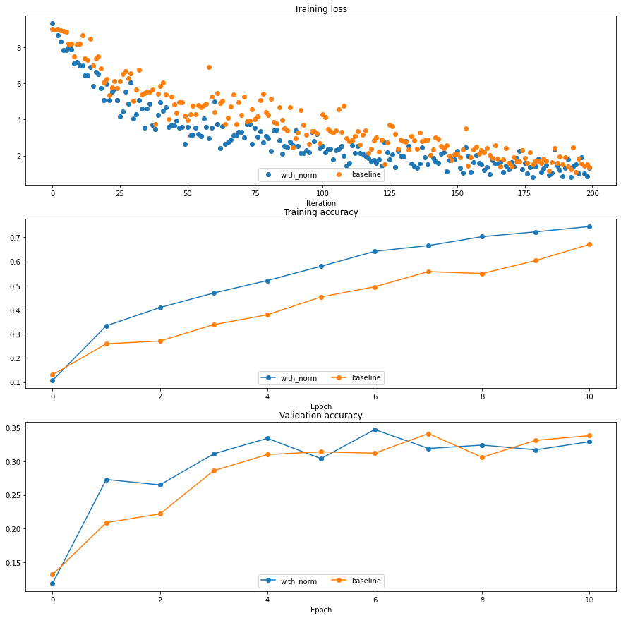
明显,带 BN 层的网准确率更高,训练速度更快
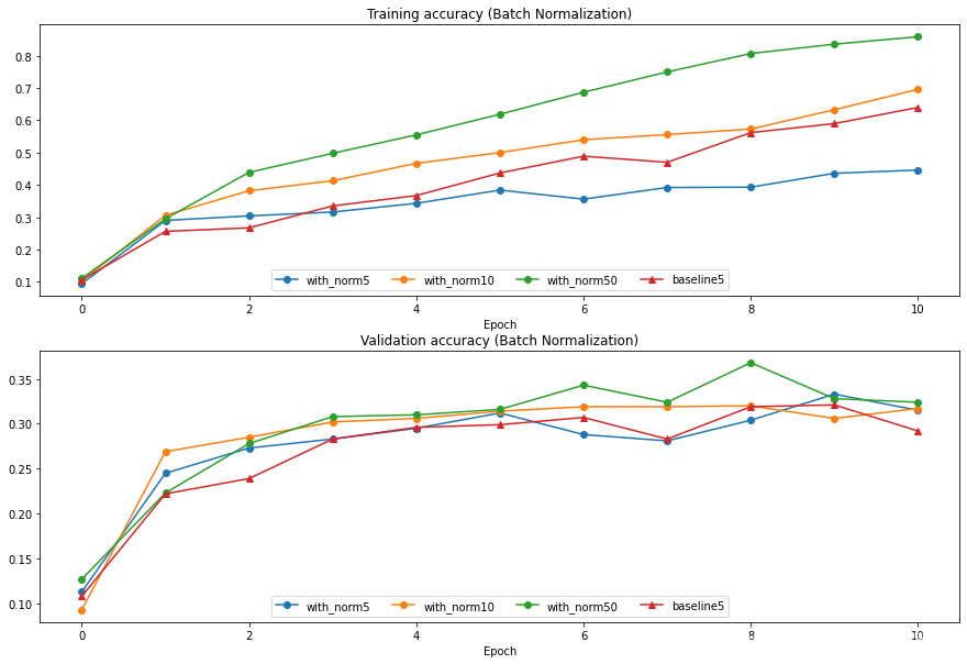
BN 层的初始化实验
我们用不同的 scales 来初始化权重,看看 BN 层的效果
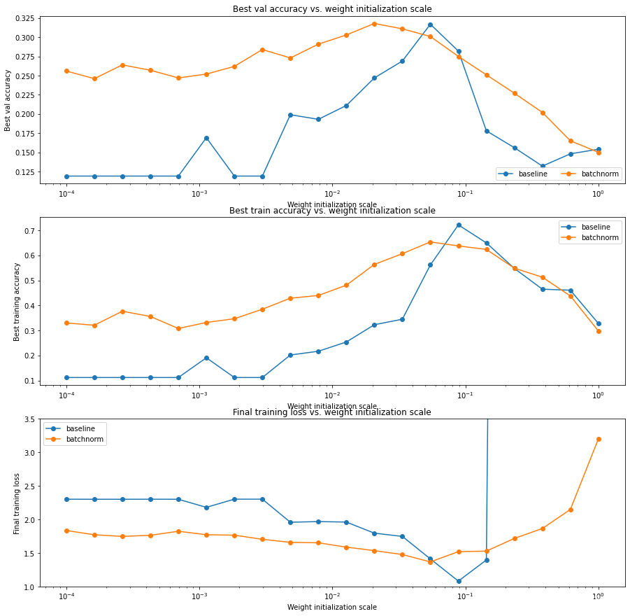
明显,带BN层的网络对权重初始化的大小不会很敏感,反而是不带BN层的非常敏感,甚至出现了梯度爆炸
Inline Question
描述一下实验结果,问权重初始化规模会不会影响到带 BN 层的模型呢?
【蒻蒟不知是否正确的回答】
由图二可以看出来,批标准化对模型的初始化敏感性较低。
第一个图显示了我们的模型过拟合,且标准化模型有比 baseline 模型更好的效果。
第三章图体现了梯度爆炸的问题,对于 baseline 模型非常明显,但是使用了批归一化的模型没有这个问题。
通常使用 BN,我们可以避免梯度消失和爆炸的问题,而且它的正则化特性可以很好的减少过拟合。
BN 层关于批量大小的实验
我们使用一下几个网络:
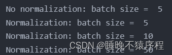
得到结果????
显然,batch_size 越大,BN 层的效果就越好
Inline Question
描述这个实验的结果。这对批量标准化和批量大小之间的关系意味着什么?为什么观察到这种关系?
【蒻蒟不知道是否正确的回答】
在训练集上,批量包含的图像越多,训练时候的准确率越大,同理可在验证集上发现这种关系。
因为如果使用小批量的数据,这些数据相比起整个数据集的均值和方差差别较大,如果批量较大我们就可以得到更为精确的近似
4. Layer Normalization
和批量归一化略有不同:
可以这样理解:
batch normalization 是用 batch 中全部的图片计算出每个像素点位置的方差和均值,然后对图像进行归一化。
later normalization 是对 batch 中的每一张图片求他的均值和方差,然后对其对应的图片进行归一化
我用画图来表示
假设输入为(N x D)

然后我们的 batch normalization 是这样求出方差和均值的
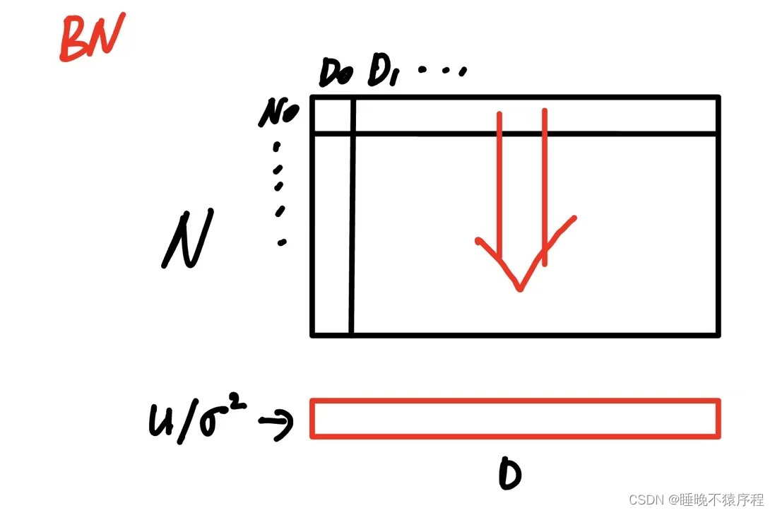
接着是 layer normalization
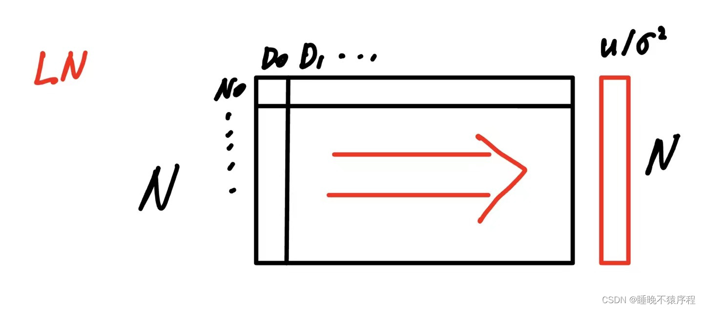
有没有发现,其实好像就是方向换了一下,可不可以通过矩阵转置然后送入 BN 来偷个懒呢?(嘿嘿)
说到做到,开始实现
4.1 Forward Pass
好吧,终究还是没有偷懒,前向传播通过偷懒可以实现,但是方向传播却不懂得怎么偷懒了iai,所以决定老老实实做了
前向传播代码如下:
def layernorm_forward(x, gamma, beta, ln_param):
    """Forward pass for layer normalization.

    During both training and test-time, the incoming data is normalized per data-point,
    before being scaled by gamma and beta parameters identical to that of batch normalization.

    Note that in contrast to batch normalization, the behavior during train and test-time for
    layer normalization are identical, and we do not need to keep track of running averages
    of any sort.

    Input:
    - x: Data of shape (N, D)
    - gamma: Scale parameter of shape (D,)
    - beta: Shift paremeter of shape (D,)
    - ln_param: Dictionary with the following keys:
        - eps: Constant for numeric stability

    Returns a tuple of:
    - out: of shape (N, D)
    - cache: A tuple of values needed in the backward pass
    """
    out, cache = None, None
    eps = ln_param.get("eps", 1e-5)
    ###########################################################################
    # TODO: Implement the training-time forward pass for layer norm.          #
    # Normalize the incoming data, and scale and  shift the normalized data   #
    #  using gamma and beta.                                                  #
    # HINT: this can be done by slightly modifying your training-time         #
    # implementation of  batch normalization, and inserting a line or two of  #
    # well-placed code. In particular, can you think of any matrix            #
    # transformations you could perform, that would enable you to copy over   #
    # the batch norm code and leave it almost unchanged?                      #
    ###########################################################################
    # *****START OF YOUR CODE (DO NOT DELETE/MODIFY THIS LINE)*****

    x_mean = np.mean(x, axis=1, keepdims=True)
    x_var = np.var(x, axis=1, keepdims=True)
    std = np.sqrt(x_var + eps)
    x_norm = (x - x_mean) / std
    out = gamma * x_norm + beta

    cache = (x, x_norm, gamma, x_mean, x_var, eps)

    # *****END OF YOUR CODE (DO NOT DELETE/MODIFY THIS LINE)*****
    ###########################################################################
    #                             END OF YOUR CODE                            #
    ###########################################################################
    return out, cache
代码详解
- 有个需要注意的点,那就是要 keepdim 保证矩阵是二位的,不然如果变成向量的话,因为 numpy 的广播机制,计算会出现问题
4.2 Backward
反向传播,还是一样画图求解,在这里我就没有再一步步推导啦,我直接写出矩阵表达式
切记注意!上面的向量都是列向量,所以需要我们保证 keepdim = True,不然运算会出现问题
来看代码吧:
def layernorm_backward(dout, cache):
    """Backward pass for layer normalization.

    For this implementation, you can heavily rely on the work you've done already
    for batch normalization.

    Inputs:
    - dout: Upstream derivatives, of shape (N, D)
    - cache: Variable of intermediates from layernorm_forward.

    Returns a tuple of:
    - dx: Gradient with respect to inputs x, of shape (N, D)
    - dgamma: Gradient with respect to scale parameter gamma, of shape (D,)
    - dbeta: Gradient with respect to shift parameter beta, of shape (D,)
    """
    dx, dgamma, dbeta = None, None, None
    ###########################################################################
    # TODO: Implement the backward pass for layer norm.                       #
    #                                                                         #
    # HINT: this can be done by slightly modifying your training-time         #
    # implementation of batch normalization. The hints to the forward pass    #
    # still apply!                                                            #
    ###########################################################################
    # *****START OF YOUR CODE (DO NOT DELETE/MODIFY THIS LINE)*****

    # (x,x_norm,gamma,x_mean,x_var,eps)
    x, x_norm, gamma, x_mean, x_var, eps = cache
    dgamma = np.sum(dout * x_norm, axis=0)  # 注意这个 *gamma 不是点乘
    dbeta = np.sum(dout, axis=0)  # 求出 dbeta

    D = 1.0 * x.shape[1]
    dldx_norm = dout * gamma
    dldvar = np.sum(-0.5 * dldx_norm * (x - x_mean) * ((x_var + eps)**-1.5),
                    axis=1)
    dldu = np.sum(-dldx_norm / np.sqrt(x_var + eps), axis=1)
    dx = dldx_norm/np.sqrt(x_var+eps)+dldu.reshape(-1, 1) / \
        D+dldvar.reshape(-1, 1)*2/D*(x-x_mean)

    # *****END OF YOUR CODE (DO NOT DELETE/MODIFY THIS LINE)*****
    ###########################################################################
    #                             END OF YOUR CODE                            #
    ###########################################################################
    return dx, dgamma, dbeta
代码详解:
- 注意看 np.sum 是向着 axis=1 方向求和的
5. 总结、预告
经过了艰苦奋斗,终于总算是把全连接网络比较难的这部分的搞定了呀,大家都不容易,奖励自己一杯奶茶吧!
下一次的内容将会是:
- Dropout 层的完成
- 完整完整的全连接网络
- 卷积神经网络卷积层,池化层的简单实现
下次见啦大家????
【注】本文章的排版以及前言的编写参考了大神@鼠标滑轮不会动,看大佬的博客受益良多!