Generalizing Linear Classification

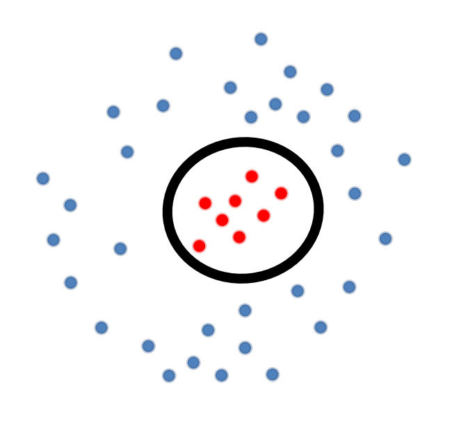
假设我们有如上图的 training data，注意到此时 $\mathcal{X} \subset \mathbb{R}^{2}$。

那么 decision boundary $g$：

\[g(\vec{x}) = w_{1} x_{1}^{2} + w_{2} x_{2}^{2} + w_{0}
\]

即，decision boundary 为某种椭圆，例如：半径为 $r$ 的圆（$w_{1} = 1, w_{2} = 1, w_{0}=-r^{2}$），如上图中的黑圈所示。我们会发现，此时 decision boundary not linear in $\vec{x}$。

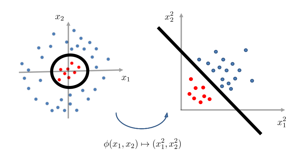
但是，$g(\vec{x}) = w_{1} x_{1}^{2} + w_{2} x_{2}^{2} + w_{0}$ 在某些空间里却是线性的：

\[\begin{align*}
g(\vec{x}) & = w_{1}x_{1}^{2} + w_{2}x_{2}^{2} + w_{0} \qquad \qquad (\text{non-linear in $x_{1}$ and $x_{2}$}) \\
& = w_{1}z_{1} + w_{2}z_{2} + w_{0} \qquad \qquad \; (\text{linear in $z_{1}$ and $z_{2}$})
\end{align*}
\]

因此，如果我们对数据进行特征变换（feature transformation）：

\[\phi(x_{1}, x_{2}) \longrightarrow (x_{1}^{2}, x_{2}^{2})
\]

那么 $g$ 在 $\phi -$ transformed feature space 中变为线性的。

Geometric view on feature transformation

Feature Transformation for Quadratic Boundaries

$\mathbb{R}^{2}-$ case

generic quadratic boundary 如下：

\[\begin{align*}
g(\vec{x}) & = w_{1} x_{1}^{2} + w_{2} x_{2}^{2} + w_{3} x_{1} x_{2} + w_{4} x_{1} + w_{5} x_{2} + w_{0} \\
& = \sum\limits_{p + q \leq 2} w^{p, q} x_{1}^{p} x_{2}^{q}
\end{align*}
\]

feature transformation 则为：

\[\phi(x_{1}, x_{2}) \longrightarrow (x_{1}^{2}, x_{2}^{2}, x_{1}x_{2}, x_{1}, x_{2}, 1)
\]

$\mathbb{R}^{d}-$ case

generic quadratic boundary 如下：

\[g(\vec{x}) = \sum\limits_{i, j = 1}^{d} \sum\limits_{p + q \leq 2} w_{i, j}^{p, q}x_{i}^{p}x_{j}^{q}
\]

feature transformation 则为：

\[\phi(x_{1}, \ldots, x_{d}) \longrightarrow (x_{1}^{2}, x_{2}^{2}, \ldots, x_{d}^{2}, x_{1}x_{2}, \ldots, x_{d-1} x_{d}, x_{1}, x_{2}, \ldots, x_{d}, 1)
\]

注意，以上的 $\mathbb{R}^{2}$ 以及下面会提到的 $\mathbb{R}^{d}$ 指的是数据的维度。

Theorem.

给定 $n$ 个互不相同的数据点：$\mathcal{X} = \left\{ \vec{x_{1}}, \vec{x_{2}}, \ldots, \vec{x_{n}} \right\}$，总是存在一个 feature transformation $\phi$，使得无论的 $\mathcal{S} = \mathcal{X} \times \mathcal{Y}$ 的 label 如何，它在 transformed space 中总是线性可分的。

Proof.

给定 $n$ 个数据点，考虑以下映射（映射至 $\mathbb{R}^{n}$）：

\[\phi(\vec{x_{i}}) \longrightarrow \begin{pmatrix}
0 \\
\vdots \\
0 \\
1 \\
0 \\
\vdots \\
0
\end{pmatrix}
\]

即，映射为一个 one-hot 向量，除第 $i$ 行处为 $1$，其它坐标处的值都为 $0$。

那么，由 linear weighting $\vec{w}^{*} = \begin{pmatrix} y_{1} \\ \vdots \\ y_{n} \end{pmatrix}$ 引出的 decision boundary 完美地分割了 input data。

解释：

证明的意思是，输入的数据有 $n$ 个。对于每一个数据点，feature transform 到一个 one-hot vector，只有这条数据在输入的 $n$ 个数据中排的位置所对应的坐标处取 $1$，其余全部取 $0$。假设输入三个数据：$\vec{x_{1}}, \vec{x_{2}}, \vec{x_{3}}$，则：

\[\phi(\vec{x_{1}}) = \begin{pmatrix}
1 \\
0 \\
0
\end{pmatrix} \qquad \phi(\vec{x_{2}}) = \begin{pmatrix}
0 \\
1 \\
0
\end{pmatrix} \qquad \phi(\vec{x_{3}}) = \begin{pmatrix}
0 \\
0 \\
1
\end{pmatrix}
\]

这样极端的操作有利有弊：

优点：

任意的问题都将变为 linear separable。
缺点：
1. 计算复杂度：
  
  generic kernel transform 的时间复杂度通常是 $\Omega(n)$，有些常用的 kernel transform 将 input space 映射到 infinite dimensional space 中。
2. 模型复杂度：
  
  模型的概括能力（generalization performance）通常随模型复杂度的下降而下降。即，若向简化模型，通常需要以牺牲模型的表现作为代价。

回顾时间复杂度 $T(n) = \Omega \big( f(n) \big)$ 的定义：

\[\exists c > 0: ~ \exists n_{0} \in \mathbb{N}^{+}: ~ \forall n \geq n_{0}: ~ T(n) \geq c \cdot f(n)
\]

那么 $\Omega(n)$ 满足：

\[\exists c > 0: ~ \exists n_{0} \in \mathbb{N}^{+}: ~ \forall n \geq n_{0}: ~ T(n) \geq cn
\]

也就是说时间复杂度最低也与 $n$ 呈线性。

The Kernel Trick (to Deal with Computation)

如果直接暴露在 generic kernel space $\phi(\vec{x_{i}})$ 中进行运算，需要时间复杂度 $\Omega(n)$。但是相对而言地，kernel space 中的两个数据点的点积可以被更快地求出，即：

\[\phi(\vec{x_{i}}) \cdot \phi(\vec{x_{j}})
\]

Examples.

在 $\mathbb{R}^{d}$ 空间中的数据的 quadratic kernel transform：
- Explicit transform：$O(d^{2})$
  
  \[\vec{x} \longrightarrow (x_{1}^{2}, \ldots, x_{d}^{2}, \sqrt{2} x_{1} x_{2}, \ldots, \sqrt{2} x_{d-1} x_{d}, \sqrt{2} x_{1}, \ldots, \sqrt{2} x_{d}, 1)
  \]
- Dot products：$O(d)$
  
  \[(1 + \vec{x_{i}} \cdot \vec{x_{j}})^{2}
  \]

径向基函数（Radial Basis Function, i.e., RBF）：
- Explicit transform：infinite dimension！
  
  \[\vec{x} \longrightarrow \Big( \big( \frac{2}{\pi} \big)^{\frac{d}{4}} e^{-||\vec{x} - \alpha||^{2}} \Big)_{\alpha \in \mathbb{R}^{d}}
  \]
- Dot products：$O(d)$
  
  \[e^{-||\vec{x_{i}} - \vec{x_{j}}||^{2}}
  \]

Kernel 变换的诀窍在于，在实现分类算法的时候只通过 “点积” 的方式接触数据。

Examples.

The Kernel Perceptron（核感知机）

回忆感知机算法，更新权重向量的核心步骤为：

\[\vec{w}^{(t)} \leftarrow \vec{w}^{(t-1)} + y \vec{x}
\]

等价地，算法可以写为：

\[\vec{w} = \sum\limits_{k=1}^{n} \alpha_{k} y_{k} \vec{x_{k}}
\]

其中，$\alpha_{k}$ 为在 $\vec{x_{k}}$ 上发生错误的次数。

因此，分类问题变为：

\[\begin{align*}
f(\vec{x}) & = \text{sign}(\vec{w} \cdot \vec{x}) \\
& = \text{sign} \big( \vec{x} \cdot \sum\limits_{k=1}^{n} \alpha_{k} y_{k} \vec{x_{k}} \big) \\
& = \text{sign} \big( \sum\limits_{k=1}^{n} \alpha_{j} y_{k} (\vec{x_{k}} \cdot \vec{x}) \big)
\end{align*}
\]

其中 $\vec{x}$ 输入函数 $f$ 的新数据向量，注意与 $\vec{x_{k}}$ 区分。

因此，在空间内的分类问题：

\[f(\vec{x}) = \text{sign} \big( \sum\limits_{k=1}^{n} \alpha_{j} y_{k} (\vec{x_{k}} \cdot \vec{x}) \big)
\]

若在 tranformed kernel space 中处理，则：

\[f\big( \phi(\vec{x}) \big) = \text{sign} \Big( \sum\limits_{k=1}^{n} \alpha_{k} y_{k} \big( \phi(\vec{x_{k}}) \cdot \phi(\vec{x}) \big) \Big)
\]

算法具体如下：

\[\begin{align*}
& \text{Initialize}: \vec{\alpha} = \vec{0} \\
& \\
& \text{for } t = 1, 2, 3, \cdots, T: \\
& \\
& \qquad \text{若存在} (\vec{x_{i}}, y) \in \mathcal{S} \text{ s.t. : } \text{sign} \Big( \sum\limits_{k=1}^{n} \alpha_{k} y_{k} \big( \phi(\vec{x_{k}}) \cdot \phi(\vec{x_{i}}) \big) \Big) \neq y_{i}: \\
& \qquad \qquad \alpha_{i} \leftarrow \alpha_{i} + 1
\end{align*}
\]

在最后注意到，$\sum\limits_{k=1}^{n} \alpha_{k} y_{k} \big( \phi(\vec{x_{k}}) \cdot \phi(\vec{x}) \big)$ 中的点积 $\phi(\vec{x_{k}}) \cdot \phi(\vec{x})$ 是相似度（similarity）的一种衡量方式，故自然能够被其它自定义的相似度衡量方式所替换。

所以，我们可以在任意自定义的非线性空间中，隐性地（implicitly）进行运算，而不需要承担可能的巨大计算量成本。