机器学习实战系列[一]:工业蒸汽量预测
- 背景介绍
火力发电的基本原理是:燃料在燃烧时加热水生成蒸汽,蒸汽压力推动汽轮机旋转,然后汽轮机带动发电机旋转,产生电能。在这一系列的能量转化中,影响发电效率的核心是锅炉的燃烧效率,即燃料燃烧加热水产生高温高压蒸汽。锅炉的燃烧效率的影响因素很多,包括锅炉的可调参数,如燃烧给量,一二次风,引风,返料风,给水水量;以及锅炉的工况,比如锅炉床温、床压,炉膛温度、压力,过热器的温度等。
- 相关描述
经脱敏后的锅炉传感器采集的数据(采集频率是分钟级别),根据锅炉的工况,预测产生的蒸汽量。
- 数据说明
数据分成训练数据(train.txt)和测试数据(test.txt),其中字段”V0”-“V37”,这38个字段是作为特征变量,”target”作为目标变量。选手利用训练数据训练出模型,预测测试数据的目标变量,排名结果依据预测结果的MSE(mean square error)。
- 结果评估
预测结果以mean square error作为评判标准。
原项目链接:https://www.heywhale.com/home/column/64141d6b1c8c8b518ba97dcc
1.数据探索性分析
import numpy as np
import pandas as pd
import matplotlib.pyplot as plt
import seaborn as sns

from scipy import stats

import warnings
warnings.filterwarnings("ignore")

%matplotlib inline
# 下载需要用到的数据集
!wget http://tianchi-media.oss-cn-beijing.aliyuncs.com/DSW/Industrial_Steam_Forecast/zhengqi_test.txt
!wget http://tianchi-media.oss-cn-beijing.aliyuncs.com/DSW/Industrial_Steam_Forecast/zhengqi_train.txt
--2023-03-23 18:10:23--  http://tianchi-media.oss-cn-beijing.aliyuncs.com/DSW/Industrial_Steam_Forecast/zhengqi_test.txt
正在解析主机 tianchi-media.oss-cn-beijing.aliyuncs.com (tianchi-media.oss-cn-beijing.aliyuncs.com)... 49.7.22.39
正在连接 tianchi-media.oss-cn-beijing.aliyuncs.com (tianchi-media.oss-cn-beijing.aliyuncs.com)|49.7.22.39|:80... 已连接。
已发出 HTTP 请求,正在等待回应... 200 OK
长度: 466959 (456K) [text/plain]
正在保存至: “zhengqi_test.txt.1”

zhengqi_test.txt.1  100%[===================>] 456.01K  --.-KB/s    in 0.04s

2023-03-23 18:10:23 (10.0 MB/s) - 已保存 “zhengqi_test.txt.1” [466959/466959])

--2023-03-23 18:10:23--  http://tianchi-media.oss-cn-beijing.aliyuncs.com/DSW/Industrial_Steam_Forecast/zhengqi_train.txt
正在解析主机 tianchi-media.oss-cn-beijing.aliyuncs.com (tianchi-media.oss-cn-beijing.aliyuncs.com)... 49.7.22.39
正在连接 tianchi-media.oss-cn-beijing.aliyuncs.com (tianchi-media.oss-cn-beijing.aliyuncs.com)|49.7.22.39|:80... 已连接。
已发出 HTTP 请求,正在等待回应... 200 OK
长度: 714370 (698K) [text/plain]
正在保存至: “zhengqi_train.txt.1”

zhengqi_train.txt.1 100%[===================>] 697.63K  --.-KB/s    in 0.04s

2023-03-23 18:10:24 (17.9 MB/s) - 已保存 “zhengqi_train.txt.1” [714370/714370])
# **读取数据文件**
# 使用Pandas库`read_csv()`函数进行数据读取,分割符为‘\t’
train_data_file = "./zhengqi_train.txt"
test_data_file =  "./zhengqi_test.txt"

train_data = pd.read_csv(train_data_file, sep='\t', encoding='utf-8')
test_data = pd.read_csv(test_data_file, sep='\t', encoding='utf-8')
1.1 查看数据信息
#查看特征变量信息
train_data.info()
<class 'pandas.core.frame.DataFrame'>
RangeIndex: 2888 entries, 0 to 2887
Data columns (total 39 columns):
 #   Column  Non-Null Count  Dtype
---  ------  --------------  -----
 0   V0      2888 non-null   float64
 1   V1      2888 non-null   float64
 2   V2      2888 non-null   float64
 3   V3      2888 non-null   float64
 4   V4      2888 non-null   float64
 5   V5      2888 non-null   float64
 6   V6      2888 non-null   float64
 7   V7      2888 non-null   float64
 8   V8      2888 non-null   float64
 9   V9      2888 non-null   float64
 10  V10     2888 non-null   float64
 11  V11     2888 non-null   float64
 12  V12     2888 non-null   float64
 13  V13     2888 non-null   float64
 14  V14     2888 non-null   float64
 15  V15     2888 non-null   float64
 16  V16     2888 non-null   float64
 17  V17     2888 non-null   float64
 18  V18     2888 non-null   float64
 19  V19     2888 non-null   float64
 20  V20     2888 non-null   float64
 21  V21     2888 non-null   float64
 22  V22     2888 non-null   float64
 23  V23     2888 non-null   float64
 24  V24     2888 non-null   float64
 25  V25     2888 non-null   float64
 26  V26     2888 non-null   float64
 27  V27     2888 non-null   float64
 28  V28     2888 non-null   float64
 29  V29     2888 non-null   float64
 30  V30     2888 non-null   float64
 31  V31     2888 non-null   float64
 32  V32     2888 non-null   float64
 33  V33     2888 non-null   float64
 34  V34     2888 non-null   float64
 35  V35     2888 non-null   float64
 36  V36     2888 non-null   float64
 37  V37     2888 non-null   float64
 38  target  2888 non-null   float64
dtypes: float64(39)
memory usage: 880.1 KB
此训练集数据共有2888个样本,数据中有V0-V37共计38个特征变量,变量类型都为数值类型,所有数据特征没有缺失值数据;
数据字段由于采用了脱敏处理,删除了特征数据的具体含义;target字段为标签变量
test_data.info()
<class 'pandas.core.frame.DataFrame'>
RangeIndex: 1925 entries, 0 to 1924
Data columns (total 38 columns):
 #   Column  Non-Null Count  Dtype
---  ------  --------------  -----
 0   V0      1925 non-null   float64
 1   V1      1925 non-null   float64
 2   V2      1925 non-null   float64
 3   V3      1925 non-null   float64
 4   V4      1925 non-null   float64
 5   V5      1925 non-null   float64
 6   V6      1925 non-null   float64
 7   V7      1925 non-null   float64
 8   V8      1925 non-null   float64
 9   V9      1925 non-null   float64
 10  V10     1925 non-null   float64
 11  V11     1925 non-null   float64
 12  V12     1925 non-null   float64
 13  V13     1925 non-null   float64
 14  V14     1925 non-null   float64
 15  V15     1925 non-null   float64
 16  V16     1925 non-null   float64
 17  V17     1925 non-null   float64
 18  V18     1925 non-null   float64
 19  V19     1925 non-null   float64
 20  V20     1925 non-null   float64
 21  V21     1925 non-null   float64
 22  V22     1925 non-null   float64
 23  V23     1925 non-null   float64
 24  V24     1925 non-null   float64
 25  V25     1925 non-null   float64
 26  V26     1925 non-null   float64
 27  V27     1925 non-null   float64
 28  V28     1925 non-null   float64
 29  V29     1925 non-null   float64
 30  V30     1925 non-null   float64
 31  V31     1925 non-null   float64
 32  V32     1925 non-null   float64
 33  V33     1925 non-null   float64
 34  V34     1925 non-null   float64
 35  V35     1925 non-null   float64
 36  V36     1925 non-null   float64
 37  V37     1925 non-null   float64
dtypes: float64(38)
memory usage: 571.6 KB
测试集数据共有1925个样本,数据中有V0-V37共计38个特征变量,变量类型都为数值类型
# 查看数据统计信息
train_data.describe()
| V0 | V1 | V2 | V3 | V4 | V5 | V6 | V7 | V8 | V9 | ... | V29 | V30 | V31 | V32 | V33 | V34 | V35 | V36 | V37 | target | |
|---|---|---|---|---|---|---|---|---|---|---|---|---|---|---|---|---|---|---|---|---|---|
| count | 2888.000000 | 2888.000000 | 2888.000000 | 2888.000000 | 2888.000000 | 2888.000000 | 2888.000000 | 2888.000000 | 2888.000000 | 2888.000000 | ... | 2888.000000 | 2888.000000 | 2888.000000 | 2888.000000 | 2888.000000 | 2888.000000 | 2888.000000 | 2888.000000 | 2888.000000 | 2888.000000 |
| mean | 0.123048 | 0.056068 | 0.289720 | -0.067790 | 0.012921 | -0.558565 | 0.182892 | 0.116155 | 0.177856 | -0.169452 | ... | 0.097648 | 0.055477 | 0.127791 | 0.020806 | 0.007801 | 0.006715 | 0.197764 | 0.030658 | -0.130330 | 0.126353 |
| std | 0.928031 | 0.941515 | 0.911236 | 0.970298 | 0.888377 | 0.517957 | 0.918054 | 0.955116 | 0.895444 | 0.953813 | ... | 1.061200 | 0.901934 | 0.873028 | 0.902584 | 1.006995 | 1.003291 | 0.985675 | 0.970812 | 1.017196 | 0.983966 |
| min | -4.335000 | -5.122000 | -3.420000 | -3.956000 | -4.742000 | -2.182000 | -4.576000 | -5.048000 | -4.692000 | -12.891000 | ... | -2.912000 | -4.507000 | -5.859000 | -4.053000 | -4.627000 | -4.789000 | -5.695000 | -2.608000 | -3.630000 | -3.044000 |
| 25% | -0.297000 | -0.226250 | -0.313000 | -0.652250 | -0.385000 | -0.853000 | -0.310000 | -0.295000 | -0.159000 | -0.390000 | ... | -0.664000 | -0.283000 | -0.170250 | -0.407250 | -0.499000 | -0.290000 | -0.202500 | -0.413000 | -0.798250 | -0.350250 |
| 50% | 0.359000 | 0.272500 | 0.386000 | -0.044500 | 0.110000 | -0.466000 | 0.388000 | 0.344000 | 0.362000 | 0.042000 | ... | -0.023000 | 0.053500 | 0.299500 | 0.039000 | -0.040000 | 0.160000 | 0.364000 | 0.137000 | -0.185500 | 0.313000 |
| 75% | 0.726000 | 0.599000 | 0.918250 | 0.624000 | 0.550250 | -0.154000 | 0.831250 | 0.782250 | 0.726000 | 0.042000 | ... | 0.745250 | 0.488000 | 0.635000 | 0.557000 | 0.462000 | 0.273000 | 0.602000 | 0.644250 | 0.495250 | 0.793250 |
| max | 2.121000 | 1.918000 | 2.828000 | 2.457000 | 2.689000 | 0.489000 | 1.895000 | 1.918000 | 2.245000 | 1.335000 | ... | 4.580000 | 2.689000 | 2.013000 | 2.395000 | 5.465000 | 5.110000 | 2.324000 | 5.238000 | 3.000000 | 2.538000 |
8 rows × 39 columns
test_data.describe()
| V0 | V1 | V2 | V3 | V4 | V5 | V6 | V7 | V8 | V9 | ... | V28 | V29 | V30 | V31 | V32 | V33 | V34 | V35 | V36 | V37 | |
|---|---|---|---|---|---|---|---|---|---|---|---|---|---|---|---|---|---|---|---|---|---|
| count | 1925.000000 | 1925.000000 | 1925.000000 | 1925.000000 | 1925.000000 | 1925.000000 | 1925.000000 | 1925.000000 | 1925.000000 | 1925.000000 | ... | 1925.000000 | 1925.000000 | 1925.000000 | 1925.000000 | 1925.000000 | 1925.000000 | 1925.000000 | 1925.000000 | 1925.000000 | 1925.000000 |
| mean | -0.184404 | -0.083912 | -0.434762 | 0.101671 | -0.019172 | 0.838049 | -0.274092 | -0.173971 | -0.266709 | 0.255114 | ... | -0.206871 | -0.146463 | -0.083215 | -0.191729 | -0.030782 | -0.011433 | -0.009985 | -0.296895 | -0.046270 | 0.195735 |
| std | 1.073333 | 1.076670 | 0.969541 | 1.034925 | 1.147286 | 0.963043 | 1.054119 | 1.040101 | 1.085916 | 1.014394 | ... | 1.064140 | 0.880593 | 1.126414 | 1.138454 | 1.130228 | 0.989732 | 0.995213 | 0.946896 | 1.040854 | 0.940599 |
| min | -4.814000 | -5.488000 | -4.283000 | -3.276000 | -4.921000 | -1.168000 | -5.649000 | -5.625000 | -6.059000 | -6.784000 | ... | -2.435000 | -2.413000 | -4.507000 | -7.698000 | -4.057000 | -4.627000 | -4.789000 | -7.477000 | -2.608000 | -3.346000 |
| 25% | -0.664000 | -0.451000 | -0.978000 | -0.644000 | -0.497000 | 0.122000 | -0.732000 | -0.509000 | -0.775000 | -0.390000 | ... | -0.453000 | -0.818000 | -0.339000 | -0.476000 | -0.472000 | -0.460000 | -0.290000 | -0.349000 | -0.593000 | -0.432000 |
| 50% | 0.065000 | 0.195000 | -0.267000 | 0.220000 | 0.118000 | 0.437000 | -0.082000 | 0.018000 | -0.004000 | 0.401000 | ... | -0.445000 | -0.199000 | 0.010000 | 0.100000 | 0.155000 | -0.040000 | 0.160000 | -0.270000 | 0.083000 | 0.152000 |
| 75% | 0.549000 | 0.589000 | 0.278000 | 0.793000 | 0.610000 | 1.928000 | 0.457000 | 0.515000 | 0.482000 | 0.904000 | ... | -0.434000 | 0.468000 | 0.447000 | 0.471000 | 0.627000 | 0.419000 | 0.273000 | 0.364000 | 0.651000 | 0.797000 |
| max | 2.100000 | 2.120000 | 1.946000 | 2.603000 | 4.475000 | 3.176000 | 1.528000 | 1.394000 | 2.408000 | 1.766000 | ... | 4.656000 | 3.022000 | 3.139000 | 1.428000 | 2.299000 | 5.465000 | 5.110000 | 1.671000 | 2.861000 | 3.021000 |
8 rows × 38 columns
上面数据显示了数据的统计信息,例如样本数,数据的均值mean,标准差std,最小值,最大值等
# 查看数据字段信息
train_data.head()
| V0 | V1 | V2 | V3 | V4 | V5 | V6 | V7 | V8 | V9 | ... | V29 | V30 | V31 | V32 | V33 | V34 | V35 | V36 | V37 | target | |
|---|---|---|---|---|---|---|---|---|---|---|---|---|---|---|---|---|---|---|---|---|---|
| 0 | 0.566 | 0.016 | -0.143 | 0.407 | 0.452 | -0.901 | -1.812 | -2.360 | -0.436 | -2.114 | ... | 0.136 | 0.109 | -0.615 | 0.327 | -4.627 | -4.789 | -5.101 | -2.608 | -3.508 | 0.175 |
| 1 | 0.968 | 0.437 | 0.066 | 0.566 | 0.194 | -0.893 | -1.566 | -2.360 | 0.332 | -2.114 | ... | -0.128 | 0.124 | 0.032 | 0.600 | -0.843 | 0.160 | 0.364 | -0.335 | -0.730 | 0.676 |
| 2 | 1.013 | 0.568 | 0.235 | 0.370 | 0.112 | -0.797 | -1.367 | -2.360 | 0.396 | -2.114 | ... | -0.009 | 0.361 | 0.277 | -0.116 | -0.843 | 0.160 | 0.364 | 0.765 | -0.589 | 0.633 |
| 3 | 0.733 | 0.368 | 0.283 | 0.165 | 0.599 | -0.679 | -1.200 | -2.086 | 0.403 | -2.114 | ... | 0.015 | 0.417 | 0.279 | 0.603 | -0.843 | -0.065 | 0.364 | 0.333 | -0.112 | 0.206 |
| 4 | 0.684 | 0.638 | 0.260 | 0.209 | 0.337 | -0.454 | -1.073 | -2.086 | 0.314 | -2.114 | ... | 0.183 | 1.078 | 0.328 | 0.418 | -0.843 | -0.215 | 0.364 | -0.280 | -0.028 | 0.384 |
5 rows × 39 columns
上面显示训练集前5条数据的基本信息,可以看到数据都是浮点型数据,数据都是数值型连续型特征
test_data.head()
| V0 | V1 | V2 | V3 | V4 | V5 | V6 | V7 | V8 | V9 | ... | V28 | V29 | V30 | V31 | V32 | V33 | V34 | V35 | V36 | V37 | |
|---|---|---|---|---|---|---|---|---|---|---|---|---|---|---|---|---|---|---|---|---|---|
| 0 | 0.368 | 0.380 | -0.225 | -0.049 | 0.379 | 0.092 | 0.550 | 0.551 | 0.244 | 0.904 | ... | -0.449 | 0.047 | 0.057 | -0.042 | 0.847 | 0.534 | -0.009 | -0.190 | -0.567 | 0.388 |
| 1 | 0.148 | 0.489 | -0.247 | -0.049 | 0.122 | -0.201 | 0.487 | 0.493 | -0.127 | 0.904 | ... | -0.443 | 0.047 | 0.560 | 0.176 | 0.551 | 0.046 | -0.220 | 0.008 | -0.294 | 0.104 |
| 2 | -0.166 | -0.062 | -0.311 | 0.046 | -0.055 | 0.063 | 0.485 | 0.493 | -0.227 | 0.904 | ... | -0.458 | -0.398 | 0.101 | 0.199 | 0.634 | 0.017 | -0.234 | 0.008 | 0.373 | 0.569 |
| 3 | 0.102 | 0.294 | -0.259 | 0.051 | -0.183 | 0.148 | 0.474 | 0.504 | 0.010 | 0.904 | ... | -0.456 | -0.398 | 1.007 | 0.137 | 1.042 | -0.040 | -0.290 | 0.008 | -0.666 | 0.391 |
| 4 | 0.300 | 0.428 | 0.208 | 0.051 | -0.033 | 0.116 | 0.408 | 0.497 | 0.155 | 0.904 | ... | -0.458 | -0.776 | 0.291 | 0.370 | 0.181 | -0.040 | -0.290 | 0.008 | -0.140 | -0.497 |
5 rows × 38 columns
1.2 可视化探索数据
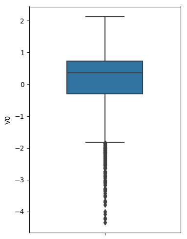
fig = plt.figure(figsize=(4, 6))  # 指定绘图对象宽度和高度
sns.boxplot(train_data['V0'],orient="v", width=0.5)
<matplotlib.axes._subplots.AxesSubplot at 0x7faf89f46950>
# 画箱式图
# column = train_data.columns.tolist()[:39]  # 列表头
# fig = plt.figure(figsize=(20, 40))  # 指定绘图对象宽度和高度
# for i in range(38):
#     plt.subplot(13, 3, i + 1)  # 13行3列子图
#     sns.boxplot(train_data[column[i]], orient="v", width=0.5)  # 箱式图
#     plt.ylabel(column[i], fontsize=8)
# plt.show()
#箱图自行打开
查看数据分布图
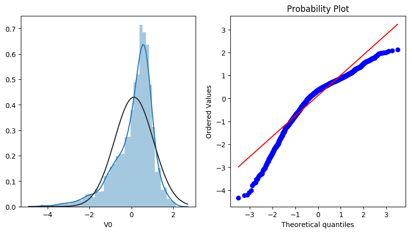
- 查看特征变量‘V0’的数据分布直方图,并绘制Q-Q图查看数据是否近似于正态分布
plt.figure(figsize=(10,5))

ax=plt.subplot(1,2,1)
sns.distplot(train_data['V0'],fit=stats.norm)
ax=plt.subplot(1,2,2)
res = stats.probplot(train_data['V0'], plot=plt)
查看查看所有数据的直方图和Q-Q图,查看训练集的数据是否近似于正态分布
# train_cols = 6
# train_rows = len(train_data.columns)
# plt.figure(figsize=(4*train_cols,4*train_rows))

# i=0
# for col in train_data.columns:
#     i+=1
#     ax=plt.subplot(train_rows,train_cols,i)
#     sns.distplot(train_data[col],fit=stats.norm)

#     i+=1
#     ax=plt.subplot(train_rows,train_cols,i)
#     res = stats.probplot(train_data[col], plot=plt)
# plt.show()
#QQ图自行打开
由上面的数据分布图信息可以看出,很多特征变量(如'V1','V9','V24','V28'等)的数据分布不是正态的,数据并不跟随对角线,后续可以使用数据变换对数据进行转换。
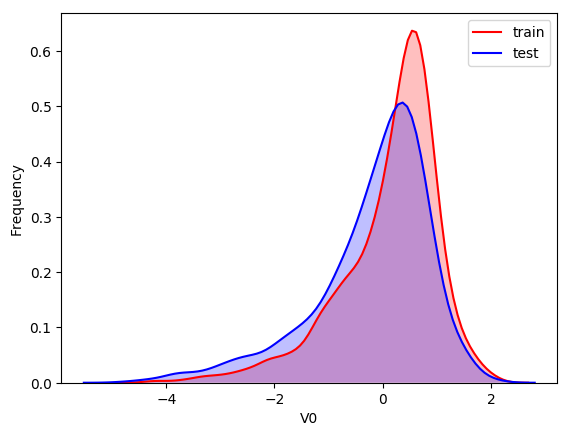
对比同一特征变量‘V0’下,训练集数据和测试集数据的分布情况,查看数据分布是否一致
ax = sns.kdeplot(train_data['V0'], color="Red", shade=True)
ax = sns.kdeplot(test_data['V0'], color="Blue", shade=True)
ax.set_xlabel('V0')
ax.set_ylabel("Frequency")
ax = ax.legend(["train","test"])
查看所有特征变量下,训练集数据和测试集数据的分布情况,分析并寻找出数据分布不一致的特征变量。
# dist_cols = 6
# dist_rows = len(test_data.columns)
# plt.figure(figsize=(4*dist_cols,4*dist_rows))

# i=1
# for col in test_data.columns:
#     ax=plt.subplot(dist_rows,dist_cols,i)
#     ax = sns.kdeplot(train_data[col], color="Red", shade=True)
#     ax = sns.kdeplot(test_data[col], color="Blue", shade=True)
#     ax.set_xlabel(col)
#     ax.set_ylabel("Frequency")
#     ax = ax.legend(["train","test"])

#     i+=1
# plt.show()
#自行打开
查看特征'V5', 'V17', 'V28', 'V22', 'V11', 'V9'数据的数据分布
drop_col = 6
drop_row = 1

plt.figure(figsize=(5*drop_col,5*drop_row))

i=1
for col in ["V5","V9","V11","V17","V22","V28"]:
    ax =plt.subplot(drop_row,drop_col,i)
    ax = sns.kdeplot(train_data[col], color="Red", shade=True)
    ax = sns.kdeplot(test_data[col], color="Blue", shade=True)
    ax.set_xlabel(col)
    ax.set_ylabel("Frequency")
    ax = ax.legend(["train","test"])

    i+=1
plt.show()
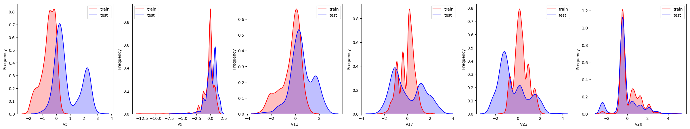
由上图的数据分布可以看到特征'V5','V9','V11','V17','V22','V28' 训练集数据与测试集数据分布不一致,会导致模型泛化能力差,采用删除此类特征方法。
drop_columns = ['V5','V9','V11','V17','V22','V28']
# 合并训练集和测试集数据,并可视化训练集和测试集数据特征分布图
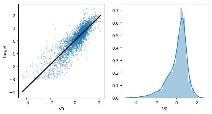
可视化线性回归关系
- 查看特征变量‘V0’与'target'变量的线性回归关系
fcols = 2
frows = 1

plt.figure(figsize=(8,4))

ax=plt.subplot(1,2,1)
sns.regplot(x='V0', y='target', data=train_data, ax=ax,
            scatter_kws={'marker':'.','s':3,'alpha':0.3},
            line_kws={'color':'k'});
plt.xlabel('V0')
plt.ylabel('target')

ax=plt.subplot(1,2,2)
sns.distplot(train_data['V0'].dropna())
plt.xlabel('V0')

plt.show()
1.2.2 查看变量间线性回归关系
# fcols = 6
# frows = len(test_data.columns)
# plt.figure(figsize=(5*fcols,4*frows))

# i=0
# for col in test_data.columns:
#     i+=1
#     ax=plt.subplot(frows,fcols,i)
#     sns.regplot(x=col, y='target', data=train_data, ax=ax,
#                 scatter_kws={'marker':'.','s':3,'alpha':0.3},
#                 line_kws={'color':'k'});
#     plt.xlabel(col)
#     plt.ylabel('target')

#     i+=1
#     ax=plt.subplot(frows,fcols,i)
#     sns.distplot(train_data[col].dropna())
    # plt.xlabel(col)
    #已注释图片生成,自行打开
1.2.2 查看特征变量的相关性
data_train1 = train_data.drop(['V5','V9','V11','V17','V22','V28'],axis=1)
train_corr = data_train1.corr()
train_corr
| V0 | V1 | V2 | V3 | V4 | V6 | V7 | V8 | V10 | V12 | ... | V29 | V30 | V31 | V32 | V33 | V34 | V35 | V36 | V37 | target | |
|---|---|---|---|---|---|---|---|---|---|---|---|---|---|---|---|---|---|---|---|---|---|
| V0 | 1.000000 | 0.908607 | 0.463643 | 0.409576 | 0.781212 | 0.189267 | 0.141294 | 0.794013 | 0.298443 | 0.751830 | ... | 0.302145 | 0.156968 | 0.675003 | 0.050951 | 0.056439 | -0.019342 | 0.138933 | 0.231417 | -0.494076 | 0.873212 |
| V1 | 0.908607 | 1.000000 | 0.506514 | 0.383924 | 0.657790 | 0.276805 | 0.205023 | 0.874650 | 0.310120 | 0.656186 | ... | 0.147096 | 0.175997 | 0.769745 | 0.085604 | 0.035129 | -0.029115 | 0.146329 | 0.235299 | -0.494043 | 0.871846 |
| V2 | 0.463643 | 0.506514 | 1.000000 | 0.410148 | 0.057697 | 0.615938 | 0.477114 | 0.703431 | 0.346006 | 0.059941 | ... | -0.275764 | 0.175943 | 0.653764 | 0.033942 | 0.050309 | -0.025620 | 0.043648 | 0.316462 | -0.734956 | 0.638878 |
| V3 | 0.409576 | 0.383924 | 0.410148 | 1.000000 | 0.315046 | 0.233896 | 0.197836 | 0.411946 | 0.321262 | 0.306397 | ... | 0.117610 | 0.043966 | 0.421954 | -0.092423 | -0.007159 | -0.031898 | 0.080034 | 0.324475 | -0.229613 | 0.512074 |
| V4 | 0.781212 | 0.657790 | 0.057697 | 0.315046 | 1.000000 | -0.117529 | -0.052370 | 0.449542 | 0.141129 | 0.927685 | ... | 0.659093 | 0.022807 | 0.447016 | -0.026186 | 0.062367 | 0.028659 | 0.100010 | 0.113609 | -0.031054 | 0.603984 |
| V6 | 0.189267 | 0.276805 | 0.615938 | 0.233896 | -0.117529 | 1.000000 | 0.917502 | 0.468233 | 0.415660 | -0.087312 | ... | -0.467980 | 0.188907 | 0.546535 | 0.144550 | 0.054210 | -0.002914 | 0.044992 | 0.433804 | -0.404817 | 0.370037 |
| V7 | 0.141294 | 0.205023 | 0.477114 | 0.197836 | -0.052370 | 0.917502 | 1.000000 | 0.389987 | 0.310982 | -0.036791 | ... | -0.311363 | 0.170113 | 0.475254 | 0.122707 | 0.034508 | -0.019103 | 0.111166 | 0.340479 | -0.292285 | 0.287815 |
| V8 | 0.794013 | 0.874650 | 0.703431 | 0.411946 | 0.449542 | 0.468233 | 0.389987 | 1.000000 | 0.419703 | 0.420557 | ... | -0.011091 | 0.150258 | 0.878072 | 0.038430 | 0.026843 | -0.036297 | 0.179167 | 0.326586 | -0.553121 | 0.831904 |
| V10 | 0.298443 | 0.310120 | 0.346006 | 0.321262 | 0.141129 | 0.415660 | 0.310982 | 0.419703 | 1.000000 | 0.140462 | ... | -0.105042 | -0.036705 | 0.560213 | -0.093213 | 0.016739 | -0.026994 | 0.026846 | 0.922190 | -0.045851 | 0.394767 |
| V12 | 0.751830 | 0.656186 | 0.059941 | 0.306397 | 0.927685 | -0.087312 | -0.036791 | 0.420557 | 0.140462 | 1.000000 | ... | 0.666775 | 0.028866 | 0.441963 | -0.007658 | 0.046674 | 0.010122 | 0.081963 | 0.112150 | -0.054827 | 0.594189 |
| V13 | 0.185144 | 0.157518 | 0.204762 | -0.003636 | 0.075993 | 0.138367 | 0.110973 | 0.153299 | -0.059553 | 0.098771 | ... | 0.008235 | 0.027328 | 0.113743 | 0.130598 | 0.157513 | 0.116944 | 0.219906 | -0.024751 | -0.379714 | 0.203373 |
| V14 | -0.004144 | -0.006268 | -0.106282 | -0.232677 | 0.023853 | 0.072911 | 0.163931 | 0.008138 | -0.077543 | 0.020069 | ... | 0.056814 | -0.004057 | 0.010989 | 0.106581 | 0.073535 | 0.043218 | 0.233523 | -0.086217 | 0.010553 | 0.008424 |
| V15 | 0.314520 | 0.164702 | -0.224573 | 0.143457 | 0.615704 | -0.431542 | -0.291272 | 0.018366 | -0.046737 | 0.642081 | ... | 0.951314 | -0.111311 | 0.011768 | -0.104618 | 0.050254 | 0.048602 | 0.100817 | -0.051861 | 0.245635 | 0.154020 |
| V16 | 0.347357 | 0.435606 | 0.782474 | 0.394517 | 0.023818 | 0.847119 | 0.752683 | 0.680031 | 0.546975 | 0.025736 | ... | -0.342210 | 0.154794 | 0.778538 | 0.041474 | 0.028878 | -0.054775 | 0.082293 | 0.551880 | -0.420053 | 0.536748 |
| V18 | 0.148622 | 0.123862 | 0.132105 | 0.022868 | 0.136022 | 0.110570 | 0.098691 | 0.093682 | -0.024693 | 0.119833 | ... | 0.053958 | 0.470341 | 0.079718 | 0.411967 | 0.512139 | 0.365410 | 0.152088 | 0.019603 | -0.181937 | 0.170721 |
| V19 | -0.100294 | -0.092673 | -0.161802 | -0.246008 | -0.205729 | 0.215290 | 0.158371 | -0.144693 | 0.074903 | -0.148319 | ... | -0.205409 | 0.100133 | -0.131542 | 0.144018 | -0.021517 | -0.079753 | -0.220737 | 0.087605 | 0.012115 | -0.114976 |
| V20 | 0.462493 | 0.459795 | 0.298385 | 0.289594 | 0.291309 | 0.136091 | 0.089399 | 0.412868 | 0.207612 | 0.271559 | ... | 0.016233 | 0.086165 | 0.326863 | 0.050699 | 0.009358 | -0.000979 | 0.048981 | 0.161315 | -0.322006 | 0.444965 |
| V21 | -0.029285 | -0.012911 | -0.030932 | 0.114373 | 0.174025 | -0.051806 | -0.065300 | -0.047839 | 0.082288 | 0.144371 | ... | 0.157097 | -0.077945 | 0.053025 | -0.159128 | -0.087561 | -0.053707 | -0.199398 | 0.047340 | 0.315470 | -0.010063 |
| V23 | 0.231136 | 0.222574 | 0.065509 | 0.081374 | 0.196530 | 0.069901 | 0.125180 | 0.174124 | -0.066537 | 0.180049 | ... | 0.116122 | 0.363963 | 0.129783 | 0.367086 | 0.183666 | 0.196681 | 0.635252 | -0.035949 | -0.187582 | 0.226331 |
| V24 | -0.324959 | -0.233556 | 0.010225 | -0.237326 | -0.529866 | 0.072418 | -0.030292 | -0.136898 | -0.029420 | -0.550881 | ... | -0.642370 | 0.033532 | -0.202097 | 0.060608 | -0.134320 | -0.095588 | -0.243738 | -0.041325 | -0.137614 | -0.264815 |
| V25 | -0.200706 | -0.070627 | 0.481785 | -0.100569 | -0.444375 | 0.438610 | 0.316744 | 0.173320 | 0.079805 | -0.448877 | ... | -0.575154 | 0.088238 | 0.201243 | 0.065501 | -0.013312 | -0.030747 | -0.093948 | 0.069302 | -0.246742 | -0.019373 |
| V26 | -0.125140 | -0.043012 | 0.035370 | -0.027685 | -0.080487 | 0.106055 | 0.160566 | 0.015724 | 0.072366 | -0.124111 | ... | -0.133694 | -0.057247 | 0.062879 | -0.004545 | -0.034596 | 0.051294 | 0.085576 | 0.064963 | 0.010880 | -0.046724 |
| V27 | 0.733198 | 0.824198 | 0.726250 | 0.392006 | 0.412083 | 0.474441 | 0.424185 | 0.901100 | 0.246085 | 0.374380 | ... | -0.032772 | 0.208074 | 0.790239 | 0.095127 | 0.030135 | -0.036123 | 0.159884 | 0.226713 | -0.617771 | 0.812585 |
| V29 | 0.302145 | 0.147096 | -0.275764 | 0.117610 | 0.659093 | -0.467980 | -0.311363 | -0.011091 | -0.105042 | 0.666775 | ... | 1.000000 | -0.122817 | -0.004364 | -0.110699 | 0.035272 | 0.035392 | 0.078588 | -0.099309 | 0.285581 | 0.123329 |
| V30 | 0.156968 | 0.175997 | 0.175943 | 0.043966 | 0.022807 | 0.188907 | 0.170113 | 0.150258 | -0.036705 | 0.028866 | ... | -0.122817 | 1.000000 | 0.114318 | 0.695725 | 0.083693 | -0.028573 | -0.027987 | 0.006961 | -0.256814 | 0.187311 |
| V31 | 0.675003 | 0.769745 | 0.653764 | 0.421954 | 0.447016 | 0.546535 | 0.475254 | 0.878072 | 0.560213 | 0.441963 | ... | -0.004364 | 0.114318 | 1.000000 | 0.016782 | 0.016733 | -0.047273 | 0.152314 | 0.510851 | -0.357785 | 0.750297 |
| V32 | 0.050951 | 0.085604 | 0.033942 | -0.092423 | -0.026186 | 0.144550 | 0.122707 | 0.038430 | -0.093213 | -0.007658 | ... | -0.110699 | 0.695725 | 0.016782 | 1.000000 | 0.105255 | 0.069300 | 0.016901 | -0.054411 | -0.162417 | 0.066606 |
| V33 | 0.056439 | 0.035129 | 0.050309 | -0.007159 | 0.062367 | 0.054210 | 0.034508 | 0.026843 | 0.016739 | 0.046674 | ... | 0.035272 | 0.083693 | 0.016733 | 0.105255 | 1.000000 | 0.719126 | 0.167597 | 0.031586 | -0.062715 | 0.077273 |
| V34 | -0.019342 | -0.029115 | -0.025620 | -0.031898 | 0.028659 | -0.002914 | -0.019103 | -0.036297 | -0.026994 | 0.010122 | ... | 0.035392 | -0.028573 | -0.047273 | 0.069300 | 0.719126 | 1.000000 | 0.233616 | -0.019032 | -0.006854 | -0.006034 |
| V35 | 0.138933 | 0.146329 | 0.043648 | 0.080034 | 0.100010 | 0.044992 | 0.111166 | 0.179167 | 0.026846 | 0.081963 | ... | 0.078588 | -0.027987 | 0.152314 | 0.016901 | 0.167597 | 0.233616 | 1.000000 | 0.025401 | -0.077991 | 0.140294 |
| V36 | 0.231417 | 0.235299 | 0.316462 | 0.324475 | 0.113609 | 0.433804 | 0.340479 | 0.326586 | 0.922190 | 0.112150 | ... | -0.099309 | 0.006961 | 0.510851 | -0.054411 | 0.031586 | -0.019032 | 0.025401 | 1.000000 | -0.039478 | 0.319309 |
| V37 | -0.494076 | -0.494043 | -0.734956 | -0.229613 | -0.031054 | -0.404817 | -0.292285 | -0.553121 | -0.045851 | -0.054827 | ... | 0.285581 | -0.256814 | -0.357785 | -0.162417 | -0.062715 | -0.006854 | -0.077991 | -0.039478 | 1.000000 | -0.565795 |
| target | 0.873212 | 0.871846 | 0.638878 | 0.512074 | 0.603984 | 0.370037 | 0.287815 | 0.831904 | 0.394767 | 0.594189 | ... | 0.123329 | 0.187311 | 0.750297 | 0.066606 | 0.077273 | -0.006034 | 0.140294 | 0.319309 | -0.565795 | 1.000000 |
33 rows × 33 columns
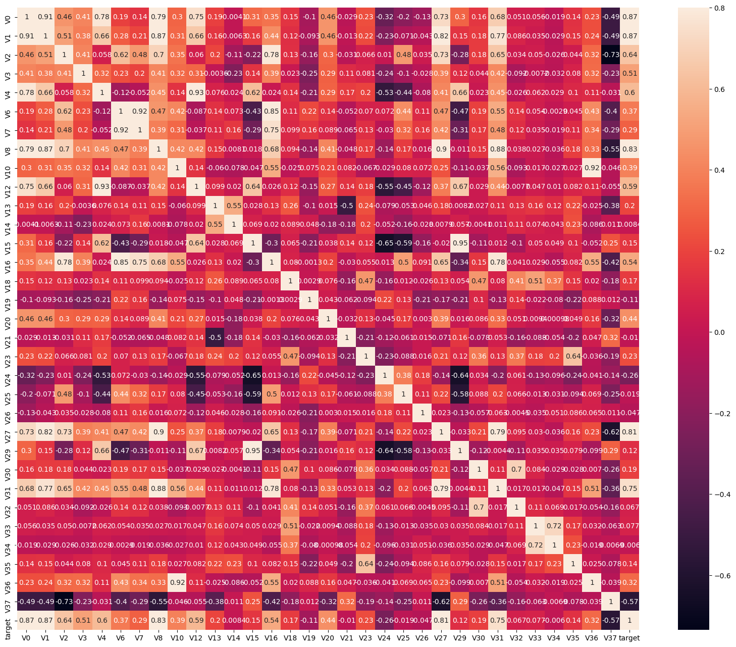
# 画出相关性热力图
ax = plt.subplots(figsize=(20, 16))#调整画布大小

ax = sns.heatmap(train_corr, vmax=.8, square=True, annot=True)#画热力图   annot=True 显示系数
# 找出相关程度
data_train1 = train_data.drop(['V5','V9','V11','V17','V22','V28'],axis=1)

plt.figure(figsize=(20, 16))  # 指定绘图对象宽度和高度
colnm = data_train1.columns.tolist()  # 列表头
mcorr = data_train1[colnm].corr(method="spearman")  # 相关系数矩阵,即给出了任意两个变量之间的相关系数
mask = np.zeros_like(mcorr, dtype=np.bool)  # 构造与mcorr同维数矩阵 为bool型
mask[np.triu_indices_from(mask)] = True  # 角分线右侧为True
cmap = sns.diverging_palette(220, 10, as_cmap=True)  # 返回matplotlib colormap对象
g = sns.heatmap(mcorr, mask=mask, cmap=cmap, square=True, annot=True, fmt='0.2f')  # 热力图(看两两相似度)
plt.show()
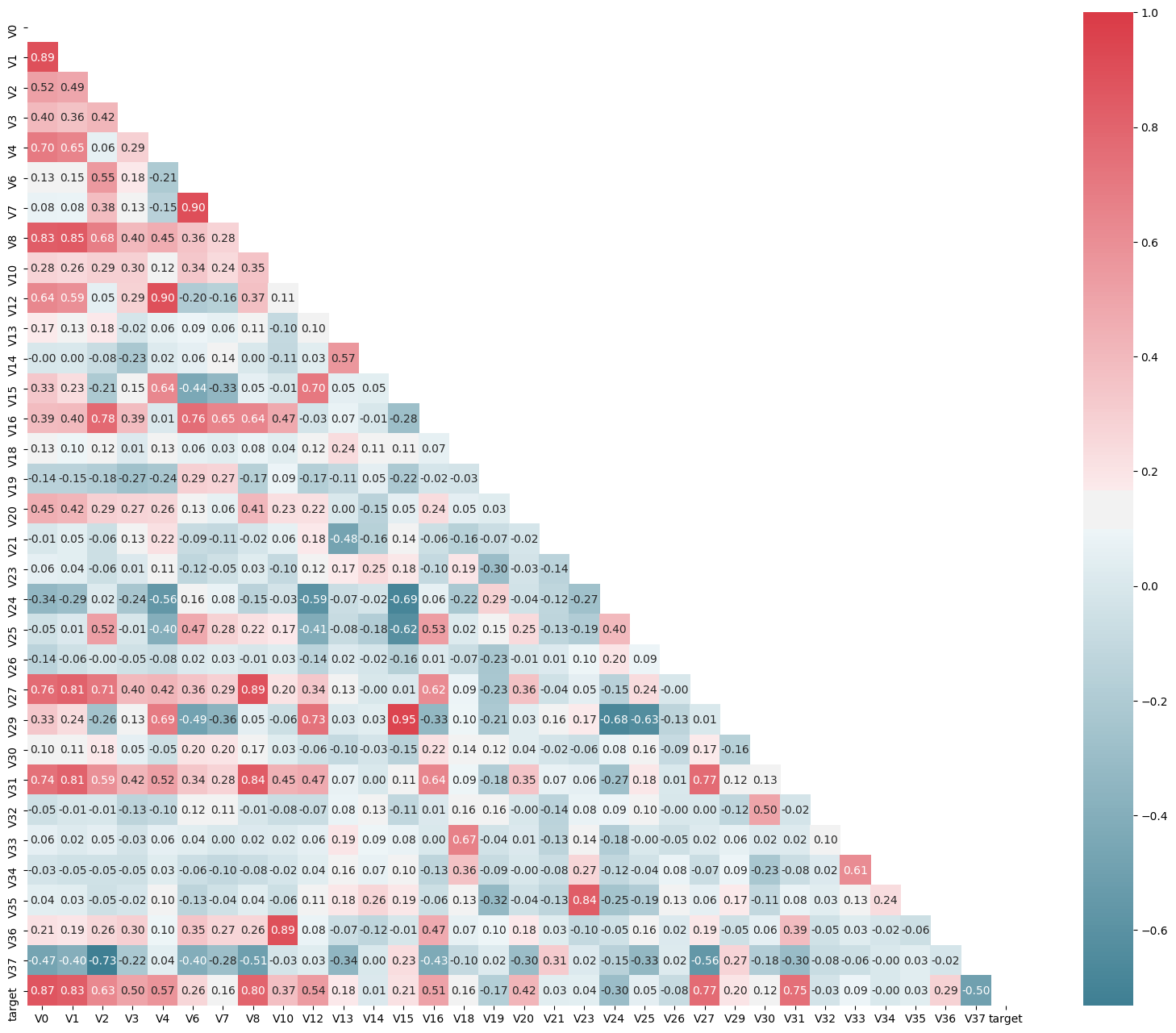
上图为所有特征变量和target变量两两之间的相关系数,由此可以看出各个特征变量V0-V37之间的相关性以及特征变量V0-V37与target的相关性。
1.2.3 查找重要变量
查找出特征变量和target变量相关系数大于0.5的特征变量
#寻找K个最相关的特征信息
k = 10 # number of variables for heatmap
cols = train_corr.nlargest(k, 'target')['target'].index

cm = np.corrcoef(train_data[cols].values.T)
hm = plt.subplots(figsize=(10, 10))#调整画布大小
#hm = sns.heatmap(cm, cbar=True, annot=True, square=True)
#g = sns.heatmap(train_data[cols].corr(),annot=True,square=True,cmap="RdYlGn")
hm = sns.heatmap(train_data[cols].corr(),annot=True,square=True)

plt.show()
threshold = 0.5

corrmat = train_data.corr()
top_corr_features = corrmat.index[abs(corrmat["target"])>threshold]
plt.figure(figsize=(10,10))
g = sns.heatmap(train_data[top_corr_features].corr(),annot=True,cmap="RdYlGn")
drop_columns.clear()
drop_columns = ['V5','V9','V11','V17','V22','V28']
# Threshold for removing correlated variables
threshold = 0.5

# Absolute value correlation matrix
corr_matrix = data_train1.corr().abs()
drop_col=corr_matrix[corr_matrix["target"]<threshold].index
#data_all.drop(drop_col, axis=1, inplace=True)
由于'V14', 'V21', 'V25', 'V26', 'V32', 'V33', 'V34'特征的相关系数值小于0.5,故认为这些特征与最终的预测target值不相关,删除这些特征变量;
#merge train_set and test_set
train_x =  train_data.drop(['target'], axis=1)

#data_all=pd.concat([train_data,test_data],axis=0,ignore_index=True)
data_all = pd.concat([train_x,test_data])


data_all.drop(drop_columns,axis=1,inplace=True)
#View data
data_all.head()
| V0 | V1 | V2 | V3 | V4 | V6 | V7 | V8 | V10 | V12 | ... | V27 | V29 | V30 | V31 | V32 | V33 | V34 | V35 | V36 | V37 | |
|---|---|---|---|---|---|---|---|---|---|---|---|---|---|---|---|---|---|---|---|---|---|
| 0 | 0.566 | 0.016 | -0.143 | 0.407 | 0.452 | -1.812 | -2.360 | -0.436 | -0.940 | -0.073 | ... | 0.168 | 0.136 | 0.109 | -0.615 | 0.327 | -4.627 | -4.789 | -5.101 | -2.608 | -3.508 |
| 1 | 0.968 | 0.437 | 0.066 | 0.566 | 0.194 | -1.566 | -2.360 | 0.332 | 0.188 | -0.134 | ... | 0.338 | -0.128 | 0.124 | 0.032 | 0.600 | -0.843 | 0.160 | 0.364 | -0.335 | -0.730 |
| 2 | 1.013 | 0.568 | 0.235 | 0.370 | 0.112 | -1.367 | -2.360 | 0.396 | 0.874 | -0.072 | ... | 0.326 | -0.009 | 0.361 | 0.277 | -0.116 | -0.843 | 0.160 | 0.364 | 0.765 | -0.589 |
| 3 | 0.733 | 0.368 | 0.283 | 0.165 | 0.599 | -1.200 | -2.086 | 0.403 | 0.011 | -0.014 | ... | 0.277 | 0.015 | 0.417 | 0.279 | 0.603 | -0.843 | -0.065 | 0.364 | 0.333 | -0.112 |
| 4 | 0.684 | 0.638 | 0.260 | 0.209 | 0.337 | -1.073 | -2.086 | 0.314 | -0.251 | 0.199 | ... | 0.332 | 0.183 | 1.078 | 0.328 | 0.418 | -0.843 | -0.215 | 0.364 | -0.280 | -0.028 |
5 rows × 32 columns
# normalise numeric columns
cols_numeric=list(data_all.columns)

def scale_minmax(col):
    return (col-col.min())/(col.max()-col.min())

data_all[cols_numeric] = data_all[cols_numeric].apply(scale_minmax,axis=0)
data_all[cols_numeric].describe()
| V0 | V1 | V2 | V3 | V4 | V6 | V7 | V8 | V10 | V12 | ... | V27 | V29 | V30 | V31 | V32 | V33 | V34 | V35 | V36 | V37 | |
|---|---|---|---|---|---|---|---|---|---|---|---|---|---|---|---|---|---|---|---|---|---|
| count | 4813.000000 | 4813.000000 | 4813.000000 | 4813.000000 | 4813.000000 | 4813.000000 | 4813.000000 | 4813.000000 | 4813.000000 | 4813.000000 | ... | 4813.000000 | 4813.000000 | 4813.000000 | 4813.000000 | 4813.000000 | 4813.000000 | 4813.000000 | 4813.000000 | 4813.000000 | 4813.000000 |
| mean | 0.694172 | 0.721357 | 0.602300 | 0.603139 | 0.523743 | 0.748823 | 0.745740 | 0.715607 | 0.348518 | 0.578507 | ... | 0.881401 | 0.388683 | 0.589459 | 0.792709 | 0.628824 | 0.458493 | 0.483790 | 0.762873 | 0.332385 | 0.545795 |
| std | 0.144198 | 0.131443 | 0.140628 | 0.152462 | 0.106430 | 0.132560 | 0.132577 | 0.118105 | 0.134882 | 0.105088 | ... | 0.128221 | 0.133475 | 0.130786 | 0.102976 | 0.155003 | 0.099095 | 0.101020 | 0.102037 | 0.127456 | 0.150356 |
| min | 0.000000 | 0.000000 | 0.000000 | 0.000000 | 0.000000 | 0.000000 | 0.000000 | 0.000000 | 0.000000 | 0.000000 | ... | 0.000000 | 0.000000 | 0.000000 | 0.000000 | 0.000000 | 0.000000 | 0.000000 | 0.000000 | 0.000000 | 0.000000 |
| 25% | 0.626676 | 0.679416 | 0.514414 | 0.503888 | 0.478182 | 0.683324 | 0.696938 | 0.664934 | 0.284327 | 0.532892 | ... | 0.888575 | 0.292445 | 0.550092 | 0.761816 | 0.562461 | 0.409037 | 0.454490 | 0.727273 | 0.270584 | 0.445647 |
| 50% | 0.729488 | 0.752497 | 0.617072 | 0.614270 | 0.535866 | 0.774125 | 0.771974 | 0.742884 | 0.366469 | 0.591635 | ... | 0.916015 | 0.375734 | 0.594428 | 0.815055 | 0.643056 | 0.454518 | 0.499949 | 0.800020 | 0.347056 | 0.539317 |
| 75% | 0.790195 | 0.799553 | 0.700464 | 0.710474 | 0.585036 | 0.842259 | 0.836405 | 0.790835 | 0.432965 | 0.641971 | ... | 0.932555 | 0.471837 | 0.650798 | 0.852229 | 0.719777 | 0.500000 | 0.511365 | 0.800020 | 0.414861 | 0.643061 |
| max | 1.000000 | 1.000000 | 1.000000 | 1.000000 | 1.000000 | 1.000000 | 1.000000 | 1.000000 | 1.000000 | 1.000000 | ... | 1.000000 | 1.000000 | 1.000000 | 1.000000 | 1.000000 | 1.000000 | 1.000000 | 1.000000 | 1.000000 | 1.000000 |
8 rows × 32 columns
#col_data_process = cols_numeric.append('target')
train_data_process = train_data[cols_numeric]
train_data_process = train_data_process[cols_numeric].apply(scale_minmax,axis=0)

test_data_process = test_data[cols_numeric]
test_data_process = test_data_process[cols_numeric].apply(scale_minmax,axis=0)
cols_numeric_left = cols_numeric[0:13]
cols_numeric_right = cols_numeric[13:]
## Check effect of Box-Cox transforms on distributions of continuous variables

train_data_process = pd.concat([train_data_process, train_data['target']], axis=1)

fcols = 6
frows = len(cols_numeric_left)
plt.figure(figsize=(4*fcols,4*frows))
i=0

for var in cols_numeric_left:
    dat = train_data_process[[var, 'target']].dropna()

    i+=1
    plt.subplot(frows,fcols,i)
    sns.distplot(dat[var] , fit=stats.norm);
    plt.title(var+' Original')
    plt.xlabel('')

    i+=1
    plt.subplot(frows,fcols,i)
    _=stats.probplot(dat[var], plot=plt)
    plt.title('skew='+'{:.4f}'.format(stats.skew(dat[var])))
    plt.xlabel('')
    plt.ylabel('')

    i+=1
    plt.subplot(frows,fcols,i)
    plt.plot(dat[var], dat['target'],'.',alpha=0.5)
    plt.title('corr='+'{:.2f}'.format(np.corrcoef(dat[var], dat['target'])[0][1]))

    i+=1
    plt.subplot(frows,fcols,i)
    trans_var, lambda_var = stats.boxcox(dat[var].dropna()+1)
    trans_var = scale_minmax(trans_var)
    sns.distplot(trans_var , fit=stats.norm);
    plt.title(var+' Tramsformed')
    plt.xlabel('')

    i+=1
    plt.subplot(frows,fcols,i)
    _=stats.probplot(trans_var, plot=plt)
    plt.title('skew='+'{:.4f}'.format(stats.skew(trans_var)))
    plt.xlabel('')
    plt.ylabel('')

    i+=1
    plt.subplot(frows,fcols,i)
    plt.plot(trans_var, dat['target'],'.',alpha=0.5)
    plt.title('corr='+'{:.2f}'.format(np.corrcoef(trans_var,dat['target'])[0][1]))
# ## Check effect of Box-Cox transforms on distributions of continuous variables

 #已注释图片生成,自行打开


# fcols = 6
# frows = len(cols_numeric_right)
# plt.figure(figsize=(4*fcols,4*frows))
# i=0

# for var in cols_numeric_right:
#     dat = train_data_process[[var, 'target']].dropna()

#     i+=1
#     plt.subplot(frows,fcols,i)
#     sns.distplot(dat[var] , fit=stats.norm);
#     plt.title(var+' Original')
#     plt.xlabel('')

#     i+=1
#     plt.subplot(frows,fcols,i)
#     _=stats.probplot(dat[var], plot=plt)
#     plt.title('skew='+'{:.4f}'.format(stats.skew(dat[var])))
#     plt.xlabel('')
#     plt.ylabel('')

#     i+=1
#     plt.subplot(frows,fcols,i)
#     plt.plot(dat[var], dat['target'],'.',alpha=0.5)
#     plt.title('corr='+'{:.2f}'.format(np.corrcoef(dat[var], dat['target'])[0][1]))

#     i+=1
#     plt.subplot(frows,fcols,i)
#     trans_var, lambda_var = stats.boxcox(dat[var].dropna()+1)
#     trans_var = scale_minmax(trans_var)
#     sns.distplot(trans_var , fit=stats.norm);
#     plt.title(var+' Tramsformed')
#     plt.xlabel('')

#     i+=1
#     plt.subplot(frows,fcols,i)
#     _=stats.probplot(trans_var, plot=plt)
#     plt.title('skew='+'{:.4f}'.format(stats.skew(trans_var)))
#     plt.xlabel('')
#     plt.ylabel('')

#     i+=1
#     plt.subplot(frows,fcols,i)
#     plt.plot(trans_var, dat['target'],'.',alpha=0.5)
#     plt.title('corr='+'{:.2f}'.format(np.corrcoef(trans_var,dat['target'])[0][1]))
2.数据特征工程
2.1数据预处理和特征处理
# 导入数据分析工具包
import numpy as np
import pandas as pd
import matplotlib.pyplot as plt
import seaborn as sns

from scipy import stats

import warnings
warnings.filterwarnings("ignore")

%matplotlib inline

# 读取数据
train_data_file = "./zhengqi_train.txt"
test_data_file =  "./zhengqi_test.txt"

train_data = pd.read_csv(train_data_file, sep='\t', encoding='utf-8')
test_data = pd.read_csv(test_data_file, sep='\t', encoding='utf-8')
train_data.describe()
#数据总览
| V0 | V1 | V2 | V3 | V4 | V5 | V6 | V7 | V8 | V9 | ... | V29 | V30 | V31 | V32 | V33 | V34 | V35 | V36 | V37 | target | |
|---|---|---|---|---|---|---|---|---|---|---|---|---|---|---|---|---|---|---|---|---|---|
| count | 2888.000000 | 2888.000000 | 2888.000000 | 2888.000000 | 2888.000000 | 2888.000000 | 2888.000000 | 2888.000000 | 2888.000000 | 2888.000000 | ... | 2888.000000 | 2888.000000 | 2888.000000 | 2888.000000 | 2888.000000 | 2888.000000 | 2888.000000 | 2888.000000 | 2888.000000 | 2888.000000 |
| mean | 0.123048 | 0.056068 | 0.289720 | -0.067790 | 0.012921 | -0.558565 | 0.182892 | 0.116155 | 0.177856 | -0.169452 | ... | 0.097648 | 0.055477 | 0.127791 | 0.020806 | 0.007801 | 0.006715 | 0.197764 | 0.030658 | -0.130330 | 0.126353 |
| std | 0.928031 | 0.941515 | 0.911236 | 0.970298 | 0.888377 | 0.517957 | 0.918054 | 0.955116 | 0.895444 | 0.953813 | ... | 1.061200 | 0.901934 | 0.873028 | 0.902584 | 1.006995 | 1.003291 | 0.985675 | 0.970812 | 1.017196 | 0.983966 |
| min | -4.335000 | -5.122000 | -3.420000 | -3.956000 | -4.742000 | -2.182000 | -4.576000 | -5.048000 | -4.692000 | -12.891000 | ... | -2.912000 | -4.507000 | -5.859000 | -4.053000 | -4.627000 | -4.789000 | -5.695000 | -2.608000 | -3.630000 | -3.044000 |
| 25% | -0.297000 | -0.226250 | -0.313000 | -0.652250 | -0.385000 | -0.853000 | -0.310000 | -0.295000 | -0.159000 | -0.390000 | ... | -0.664000 | -0.283000 | -0.170250 | -0.407250 | -0.499000 | -0.290000 | -0.202500 | -0.413000 | -0.798250 | -0.350250 |
| 50% | 0.359000 | 0.272500 | 0.386000 | -0.044500 | 0.110000 | -0.466000 | 0.388000 | 0.344000 | 0.362000 | 0.042000 | ... | -0.023000 | 0.053500 | 0.299500 | 0.039000 | -0.040000 | 0.160000 | 0.364000 | 0.137000 | -0.185500 | 0.313000 |
| 75% | 0.726000 | 0.599000 | 0.918250 | 0.624000 | 0.550250 | -0.154000 | 0.831250 | 0.782250 | 0.726000 | 0.042000 | ... | 0.745250 | 0.488000 | 0.635000 | 0.557000 | 0.462000 | 0.273000 | 0.602000 | 0.644250 | 0.495250 | 0.793250 |
| max | 2.121000 | 1.918000 | 2.828000 | 2.457000 | 2.689000 | 0.489000 | 1.895000 | 1.918000 | 2.245000 | 1.335000 | ... | 4.580000 | 2.689000 | 2.013000 | 2.395000 | 5.465000 | 5.110000 | 2.324000 | 5.238000 | 3.000000 | 2.538000 |
8 rows × 39 columns
2.1.1 异常值分析
#异常值分析
plt.figure(figsize=(18, 10))
plt.boxplot(x=train_data.values,labels=train_data.columns)
plt.hlines([-7.5, 7.5], 0, 40, colors='r')
plt.show()
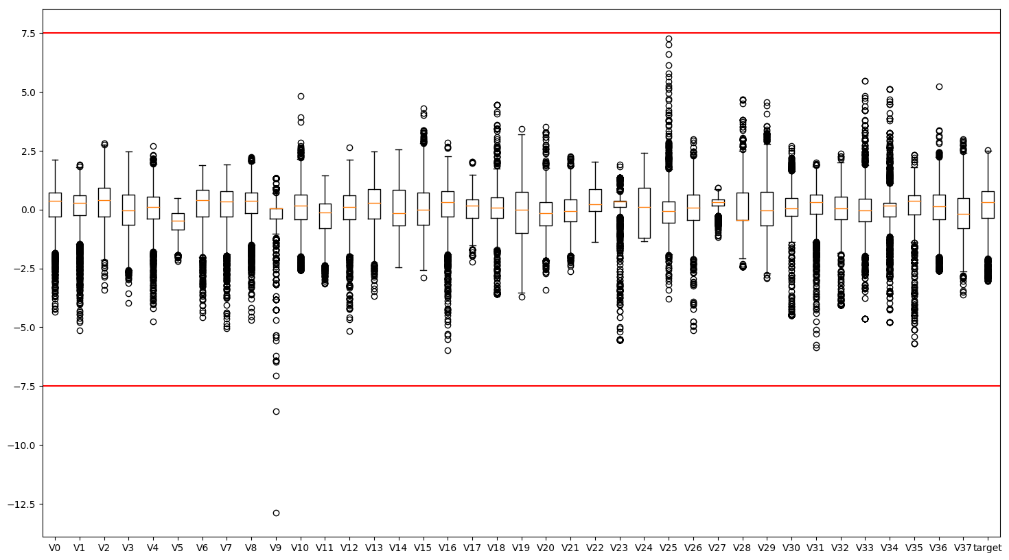
## 删除异常值
train_data = train_data[train_data['V9']>-7.5]
train_data.describe()
| V0 | V1 | V2 | V3 | V4 | V5 | V6 | V7 | V8 | V9 | ... | V29 | V30 | V31 | V32 | V33 | V34 | V35 | V36 | V37 | target | |
|---|---|---|---|---|---|---|---|---|---|---|---|---|---|---|---|---|---|---|---|---|---|
| count | 2886.000000 | 2886.000000 | 2886.000000 | 2886.000000 | 2886.000000 | 2886.000000 | 2886.000000 | 2886.000000 | 2886.000000 | 2886.00000 | ... | 2886.000000 | 2886.000000 | 2886.000000 | 2886.000000 | 2886.000000 | 2886.000000 | 2886.000000 | 2886.000000 | 2886.000000 | 2886.000000 |
| mean | 0.123725 | 0.056856 | 0.290340 | -0.068364 | 0.012254 | -0.558971 | 0.183273 | 0.116274 | 0.178138 | -0.16213 | ... | 0.097019 | 0.058619 | 0.127617 | 0.023626 | 0.008271 | 0.006959 | 0.198513 | 0.030099 | -0.131957 | 0.127451 |
| std | 0.927984 | 0.941269 | 0.911231 | 0.970357 | 0.888037 | 0.517871 | 0.918211 | 0.955418 | 0.895552 | 0.91089 | ... | 1.060824 | 0.894311 | 0.873300 | 0.896509 | 1.007175 | 1.003411 | 0.985058 | 0.970258 | 1.015666 | 0.983144 |
| min | -4.335000 | -5.122000 | -3.420000 | -3.956000 | -4.742000 | -2.182000 | -4.576000 | -5.048000 | -4.692000 | -7.07100 | ... | -2.912000 | -4.507000 | -5.859000 | -4.053000 | -4.627000 | -4.789000 | -5.695000 | -2.608000 | -3.630000 | -3.044000 |
| 25% | -0.292000 | -0.224250 | -0.310000 | -0.652750 | -0.385000 | -0.853000 | -0.310000 | -0.295000 | -0.158750 | -0.39000 | ... | -0.664000 | -0.282000 | -0.170750 | -0.405000 | -0.499000 | -0.290000 | -0.199750 | -0.412750 | -0.798750 | -0.347500 |
| 50% | 0.359500 | 0.273000 | 0.386000 | -0.045000 | 0.109500 | -0.466000 | 0.388500 | 0.345000 | 0.362000 | 0.04200 | ... | -0.023000 | 0.054500 | 0.299500 | 0.040000 | -0.040000 | 0.160000 | 0.364000 | 0.137000 | -0.186000 | 0.314000 |
| 75% | 0.726000 | 0.599000 | 0.918750 | 0.623500 | 0.550000 | -0.154000 | 0.831750 | 0.782750 | 0.726000 | 0.04200 | ... | 0.745000 | 0.488000 | 0.635000 | 0.557000 | 0.462000 | 0.273000 | 0.602000 | 0.643750 | 0.493000 | 0.793750 |
| max | 2.121000 | 1.918000 | 2.828000 | 2.457000 | 2.689000 | 0.489000 | 1.895000 | 1.918000 | 2.245000 | 1.33500 | ... | 4.580000 | 2.689000 | 2.013000 | 2.395000 | 5.465000 | 5.110000 | 2.324000 | 5.238000 | 3.000000 | 2.538000 |
8 rows × 39 columns
test_data.describe()
| V0 | V1 | V2 | V3 | V4 | V5 | V6 | V7 | V8 | V9 | ... | V28 | V29 | V30 | V31 | V32 | V33 | V34 | V35 | V36 | V37 | |
|---|---|---|---|---|---|---|---|---|---|---|---|---|---|---|---|---|---|---|---|---|---|
| count | 1925.000000 | 1925.000000 | 1925.000000 | 1925.000000 | 1925.000000 | 1925.000000 | 1925.000000 | 1925.000000 | 1925.000000 | 1925.000000 | ... | 1925.000000 | 1925.000000 | 1925.000000 | 1925.000000 | 1925.000000 | 1925.000000 | 1925.000000 | 1925.000000 | 1925.000000 | 1925.000000 |
| mean | -0.184404 | -0.083912 | -0.434762 | 0.101671 | -0.019172 | 0.838049 | -0.274092 | -0.173971 | -0.266709 | 0.255114 | ... | -0.206871 | -0.146463 | -0.083215 | -0.191729 | -0.030782 | -0.011433 | -0.009985 | -0.296895 | -0.046270 | 0.195735 |
| std | 1.073333 | 1.076670 | 0.969541 | 1.034925 | 1.147286 | 0.963043 | 1.054119 | 1.040101 | 1.085916 | 1.014394 | ... | 1.064140 | 0.880593 | 1.126414 | 1.138454 | 1.130228 | 0.989732 | 0.995213 | 0.946896 | 1.040854 | 0.940599 |
| min | -4.814000 | -5.488000 | -4.283000 | -3.276000 | -4.921000 | -1.168000 | -5.649000 | -5.625000 | -6.059000 | -6.784000 | ... | -2.435000 | -2.413000 | -4.507000 | -7.698000 | -4.057000 | -4.627000 | -4.789000 | -7.477000 | -2.608000 | -3.346000 |
| 25% | -0.664000 | -0.451000 | -0.978000 | -0.644000 | -0.497000 | 0.122000 | -0.732000 | -0.509000 | -0.775000 | -0.390000 | ... | -0.453000 | -0.818000 | -0.339000 | -0.476000 | -0.472000 | -0.460000 | -0.290000 | -0.349000 | -0.593000 | -0.432000 |
| 50% | 0.065000 | 0.195000 | -0.267000 | 0.220000 | 0.118000 | 0.437000 | -0.082000 | 0.018000 | -0.004000 | 0.401000 | ... | -0.445000 | -0.199000 | 0.010000 | 0.100000 | 0.155000 | -0.040000 | 0.160000 | -0.270000 | 0.083000 | 0.152000 |
| 75% | 0.549000 | 0.589000 | 0.278000 | 0.793000 | 0.610000 | 1.928000 | 0.457000 | 0.515000 | 0.482000 | 0.904000 | ... | -0.434000 | 0.468000 | 0.447000 | 0.471000 | 0.627000 | 0.419000 | 0.273000 | 0.364000 | 0.651000 | 0.797000 |
| max | 2.100000 | 2.120000 | 1.946000 | 2.603000 | 4.475000 | 3.176000 | 1.528000 | 1.394000 | 2.408000 | 1.766000 | ... | 4.656000 | 3.022000 | 3.139000 | 1.428000 | 2.299000 | 5.465000 | 5.110000 | 1.671000 | 2.861000 | 3.021000 |
8 rows × 38 columns
2.1.2 归一化处理
from sklearn import preprocessing

features_columns = [col for col in train_data.columns if col not in ['target']]

min_max_scaler = preprocessing.MinMaxScaler()

min_max_scaler = min_max_scaler.fit(train_data[features_columns])

train_data_scaler = min_max_scaler.transform(train_data[features_columns])
test_data_scaler = min_max_scaler.transform(test_data[features_columns])

train_data_scaler = pd.DataFrame(train_data_scaler)
train_data_scaler.columns = features_columns

test_data_scaler = pd.DataFrame(test_data_scaler)
test_data_scaler.columns = features_columns

train_data_scaler['target'] = train_data['target']
train_data_scaler.describe()

test_data_scaler.describe()
| V0 | V1 | V2 | V3 | V4 | V5 | V6 | V7 | V8 | V9 | ... | V28 | V29 | V30 | V31 | V32 | V33 | V34 | V35 | V36 | V37 | |
|---|---|---|---|---|---|---|---|---|---|---|---|---|---|---|---|---|---|---|---|---|---|
| count | 1925.000000 | 1925.000000 | 1925.000000 | 1925.000000 | 1925.000000 | 1925.000000 | 1925.000000 | 1925.000000 | 1925.000000 | 1925.000000 | ... | 1925.000000 | 1925.000000 | 1925.000000 | 1925.000000 | 1925.000000 | 1925.000000 | 1925.000000 | 1925.000000 | 1925.000000 | 1925.000000 |
| mean | 0.642905 | 0.715637 | 0.477791 | 0.632726 | 0.635558 | 1.130681 | 0.664798 | 0.699688 | 0.637926 | 0.871534 | ... | 0.313556 | 0.369132 | 0.614756 | 0.719928 | 0.623793 | 0.457349 | 0.482778 | 0.673164 | 0.326501 | 0.577034 |
| std | 0.166253 | 0.152936 | 0.155176 | 0.161379 | 0.154392 | 0.360555 | 0.162899 | 0.149311 | 0.156540 | 0.120675 | ... | 0.149752 | 0.117538 | 0.156533 | 0.144621 | 0.175284 | 0.098071 | 0.100537 | 0.118082 | 0.132661 | 0.141870 |
| min | -0.074195 | -0.051989 | -0.138124 | 0.106035 | -0.024088 | 0.379633 | -0.165817 | -0.082831 | -0.197059 | 0.034142 | ... | 0.000000 | 0.066604 | 0.000000 | -0.233613 | -0.000620 | 0.000000 | 0.000000 | -0.222222 | 0.000000 | 0.042836 |
| 25% | 0.568618 | 0.663494 | 0.390845 | 0.516451 | 0.571256 | 0.862598 | 0.594035 | 0.651593 | 0.564653 | 0.794789 | ... | 0.278919 | 0.279498 | 0.579211 | 0.683816 | 0.555366 | 0.412901 | 0.454490 | 0.666667 | 0.256819 | 0.482353 |
| 50% | 0.681537 | 0.755256 | 0.504641 | 0.651177 | 0.654017 | 0.980532 | 0.694483 | 0.727247 | 0.675796 | 0.888889 | ... | 0.280045 | 0.362120 | 0.627710 | 0.756987 | 0.652605 | 0.454518 | 0.499949 | 0.676518 | 0.342977 | 0.570437 |
| 75% | 0.756506 | 0.811222 | 0.591869 | 0.740527 | 0.720226 | 1.538750 | 0.777778 | 0.798593 | 0.745856 | 0.948727 | ... | 0.281593 | 0.451148 | 0.688438 | 0.804116 | 0.725806 | 0.500000 | 0.511365 | 0.755580 | 0.415371 | 0.667722 |
| max | 0.996747 | 1.028693 | 0.858835 | 1.022766 | 1.240345 | 2.005990 | 0.943285 | 0.924777 | 1.023497 | 1.051273 | ... | 0.997889 | 0.792045 | 1.062535 | 0.925686 | 0.985112 | 1.000000 | 1.000000 | 0.918568 | 0.697043 | 1.003167 |
8 rows × 38 columns
#查看数据集情况
dist_cols = 6
dist_rows = len(test_data_scaler.columns)

plt.figure(figsize=(4*dist_cols,4*dist_rows))


for i, col in enumerate(test_data_scaler.columns):
    ax=plt.subplot(dist_rows,dist_cols,i+1)
    ax = sns.kdeplot(train_data_scaler[col], color="Red", shade=True)
    ax = sns.kdeplot(test_data_scaler[col], color="Blue", shade=True)
    ax.set_xlabel(col)
    ax.set_ylabel("Frequency")
    ax = ax.legend(["train","test"])

# plt.show()
 #已注释图片生成,自行打开
查看特征'V5', 'V17', 'V28', 'V22', 'V11', 'V9'数据的数据分布
drop_col = 6
drop_row = 1

plt.figure(figsize=(5*drop_col,5*drop_row))

for i, col in enumerate(["V5","V9","V11","V17","V22","V28"]):
    ax =plt.subplot(drop_row,drop_col,i+1)
    ax = sns.kdeplot(train_data_scaler[col], color="Red", shade=True)
    ax= sns.kdeplot(test_data_scaler[col], color="Blue", shade=True)
    ax.set_xlabel(col)
    ax.set_ylabel("Frequency")
    ax = ax.legend(["train","test"])
plt.show()
这几个特征下,训练集的数据和测试集的数据分布不一致,会影响模型的泛化能力,故删除这些特征
3.1.3 特征相关性
plt.figure(figsize=(20, 16))
column = train_data_scaler.columns.tolist()
mcorr = train_data_scaler[column].corr(method="spearman")
mask = np.zeros_like(mcorr, dtype=np.bool)
mask[np.triu_indices_from(mask)] = True
cmap = sns.diverging_palette(220, 10, as_cmap=True)
g = sns.heatmap(mcorr, mask=mask, cmap=cmap, square=True, annot=True, fmt='0.2f')
plt.show()
2.2 特征降维
mcorr=mcorr.abs()
numerical_corr=mcorr[mcorr['target']>0.1]['target']
print(numerical_corr.sort_values(ascending=False))

index0 = numerical_corr.sort_values(ascending=False).index
print(train_data_scaler[index0].corr('spearman'))
target    1.000000
V0        0.712403
V31       0.711636
V1        0.682909
V8        0.679469
V27       0.657398
V2        0.585850
V16       0.545793
V3        0.501622
V4        0.478683
V12       0.460300
V10       0.448682
V36       0.425991
V37       0.376443
V24       0.305526
V5        0.286076
V6        0.280195
V20       0.278381
V11       0.234551
V15       0.221290
V29       0.190109
V7        0.185321
V19       0.180111
V18       0.149741
V13       0.149199
V17       0.126262
V22       0.112743
V30       0.101378
Name: target, dtype: float64
          target        V0       V31        V1        V8       V27        V2  \
target  1.000000  0.712403  0.711636  0.682909  0.679469  0.657398  0.585850
V0      0.712403  1.000000  0.739116  0.894116  0.832151  0.763128  0.516817
V31     0.711636  0.739116  1.000000  0.807585  0.841469  0.765750  0.589890
V1      0.682909  0.894116  0.807585  1.000000  0.849034  0.807102  0.490239
V8      0.679469  0.832151  0.841469  0.849034  1.000000  0.887119  0.676417
V27     0.657398  0.763128  0.765750  0.807102  0.887119  1.000000  0.709534
V2      0.585850  0.516817  0.589890  0.490239  0.676417  0.709534  1.000000
V16     0.545793  0.388852  0.642309  0.396122  0.642156  0.620981  0.783643
V3      0.501622  0.401150  0.420134  0.363749  0.400915  0.402468  0.417190
V4      0.478683  0.697430  0.521226  0.651615  0.455801  0.424260  0.062134
V12     0.460300  0.640696  0.471528  0.596173  0.368572  0.336190  0.055734
V10     0.448682  0.279350  0.445335  0.255763  0.351127  0.203066  0.292769
V36     0.425991  0.214930  0.390250  0.192985  0.263291  0.186131  0.259475
V37    -0.376443 -0.472200 -0.301906 -0.397080 -0.507057 -0.557098 -0.731786
V24    -0.305526 -0.336325 -0.267968 -0.289742 -0.148323 -0.153834  0.018458
V5     -0.286076 -0.356704 -0.162304 -0.242776 -0.188993 -0.222596 -0.324464
V6      0.280195  0.131507  0.340145  0.147037  0.355064  0.356526  0.546921
V20     0.278381  0.444939  0.349530  0.421987  0.408853  0.361040  0.293635
V11    -0.234551 -0.333101 -0.131425 -0.221910 -0.161792 -0.190952 -0.271868
V15     0.221290  0.334135  0.110674  0.230395  0.054701  0.007156 -0.206499
V29     0.190109  0.334603  0.121833  0.240964  0.050211  0.006048 -0.255559
V7      0.185321  0.075732  0.277283  0.082766  0.278231  0.290620  0.378984
V19    -0.180111 -0.144295 -0.183185 -0.146559 -0.170237 -0.228613 -0.179416
V18     0.149741  0.132143  0.094678  0.093688  0.079592  0.091660  0.114929
V13     0.149199  0.173861  0.071517  0.134595  0.105380  0.126831  0.180477
V17     0.126262  0.055024  0.115056  0.081446  0.102544  0.036520 -0.050935
V22    -0.112743 -0.076698 -0.106450 -0.072848 -0.078333 -0.111196 -0.241206
V30     0.101378  0.099242  0.131453  0.109216  0.165204  0.167073  0.176236

             V16        V3        V4  ...       V11       V15       V29  \
target  0.545793  0.501622  0.478683  ... -0.234551  0.221290  0.190109
V0      0.388852  0.401150  0.697430  ... -0.333101  0.334135  0.334603
V31     0.642309  0.420134  0.521226  ... -0.131425  0.110674  0.121833
V1      0.396122  0.363749  0.651615  ... -0.221910  0.230395  0.240964
V8      0.642156  0.400915  0.455801  ... -0.161792  0.054701  0.050211
V27     0.620981  0.402468  0.424260  ... -0.190952  0.007156  0.006048
V2      0.783643  0.417190  0.062134  ... -0.271868 -0.206499 -0.255559
V16     1.000000  0.388886  0.009749  ... -0.088716 -0.280952 -0.327558
V3      0.388886  1.000000  0.294049  ... -0.126924  0.145291  0.128079
V4      0.009749  0.294049  1.000000  ... -0.164113  0.641180  0.692626
V12    -0.024541  0.286500  0.897807  ... -0.232228  0.703861  0.732617
V10     0.473009  0.295181  0.123829  ...  0.049969 -0.014449 -0.060440
V36     0.469130  0.299063  0.099359  ... -0.017805 -0.012844 -0.051097
V37    -0.431507 -0.219751  0.040396  ...  0.455998  0.234751  0.273926
V24     0.064523 -0.237022 -0.558334  ...  0.170969 -0.687353 -0.677833
V5     -0.045495 -0.230466 -0.248061  ...  0.797583 -0.250027 -0.233233
V6      0.760362  0.181135 -0.204780  ... -0.170545 -0.443436 -0.486682
V20     0.239572  0.270647  0.257815  ... -0.138684  0.050867  0.035022
V11    -0.088716 -0.126924 -0.164113  ...  1.000000 -0.123004 -0.120982
V15    -0.280952  0.145291  0.641180  ... -0.123004  1.000000  0.947360
V29    -0.327558  0.128079  0.692626  ... -0.120982  0.947360  1.000000
V7      0.651907  0.132564 -0.150577  ... -0.097623 -0.335054 -0.360490
V19    -0.019645 -0.265940 -0.237529  ... -0.094150 -0.215364 -0.212691
V18     0.066147  0.014697  0.135792  ... -0.153625  0.109030  0.098474
V13     0.074214 -0.019453  0.061801  ... -0.436341  0.047845  0.024514
V17     0.172978  0.067720  0.060753  ...  0.192222 -0.004555 -0.006498
V22    -0.091204 -0.305218  0.021174  ...  0.079577  0.069993  0.072070
V30     0.217428  0.055660 -0.053976  ... -0.102750 -0.147541 -0.161966

              V7       V19       V18       V13       V17       V22       V30
target  0.185321 -0.180111  0.149741  0.149199  0.126262 -0.112743  0.101378
V0      0.075732 -0.144295  0.132143  0.173861  0.055024 -0.076698  0.099242
V31     0.277283 -0.183185  0.094678  0.071517  0.115056 -0.106450  0.131453
V1      0.082766 -0.146559  0.093688  0.134595  0.081446 -0.072848  0.109216
V8      0.278231 -0.170237  0.079592  0.105380  0.102544 -0.078333  0.165204
V27     0.290620 -0.228613  0.091660  0.126831  0.036520 -0.111196  0.167073
V2      0.378984 -0.179416  0.114929  0.180477 -0.050935 -0.241206  0.176236
V16     0.651907 -0.019645  0.066147  0.074214  0.172978 -0.091204  0.217428
V3      0.132564 -0.265940  0.014697 -0.019453  0.067720 -0.305218  0.055660
V4     -0.150577 -0.237529  0.135792  0.061801  0.060753  0.021174 -0.053976
V12    -0.157087 -0.174034  0.125965  0.102293  0.012429 -0.004863 -0.054432
V10     0.242818  0.089046  0.038237 -0.100776  0.258885 -0.132951  0.027257
V36     0.268044  0.099034  0.066478 -0.068582  0.298962 -0.136943  0.056802
V37    -0.284305  0.025241 -0.097699 -0.344661  0.052673  0.110455 -0.176127
V24     0.076407  0.287262 -0.221117 -0.073906  0.094367  0.081279  0.079363
V5      0.118541  0.247903 -0.191786 -0.408978  0.342555  0.143785  0.020252
V6      0.904614  0.292661  0.061109  0.088866  0.094702 -0.102842  0.201834
V20     0.064205  0.029483  0.050529  0.004600  0.061369 -0.092706  0.035036
V11    -0.097623 -0.094150 -0.153625 -0.436341  0.192222  0.079577 -0.102750
V15    -0.335054 -0.215364  0.109030  0.047845 -0.004555  0.069993 -0.147541
V29    -0.360490 -0.212691  0.098474  0.024514 -0.006498  0.072070 -0.161966
V7      1.000000  0.269472  0.032519  0.059724  0.178034  0.058178  0.196347
V19     0.269472  1.000000 -0.034215 -0.106162  0.250114  0.075582  0.120766
V18     0.032519 -0.034215  1.000000  0.242008 -0.073678  0.016819  0.133708
V13     0.059724 -0.106162  0.242008  1.000000 -0.108020  0.348432 -0.097178
V17     0.178034  0.250114 -0.073678 -0.108020  1.000000  0.363785  0.057480
V22     0.058178  0.075582  0.016819  0.348432  0.363785  1.000000 -0.054570
V30     0.196347  0.120766  0.133708 -0.097178  0.057480 -0.054570  1.000000

[28 rows x 28 columns]
2.2.1 相关性初筛
features_corr = numerical_corr.sort_values(ascending=False).reset_index()
features_corr.columns = ['features_and_target', 'corr']
features_corr_select = features_corr[features_corr['corr']>0.3] # 筛选出大于相关性大于0.3的特征
print(features_corr_select)
select_features = [col for col in features_corr_select['features_and_target'] if col not in ['target']]
new_train_data_corr_select = train_data_scaler[select_features+['target']]
new_test_data_corr_select = test_data_scaler[select_features]
   features_and_target      corr
0               target  1.000000
1                   V0  0.712403
2                  V31  0.711636
3                   V1  0.682909
4                   V8  0.679469
5                  V27  0.657398
6                   V2  0.585850
7                  V16  0.545793
8                   V3  0.501622
9                   V4  0.478683
10                 V12  0.460300
11                 V10  0.448682
12                 V36  0.425991
13                 V37  0.376443
14                 V24  0.305526
2.2.2 多重共线性分析
!pip install statsmodels -i https://pypi.tuna.tsinghua.edu.cn/simple
Looking in indexes: https://pypi.tuna.tsinghua.edu.cn/simple
Requirement already satisfied: statsmodels in /opt/conda/envs/python35-paddle120-env/lib/python3.7/site-packages (0.13.5)
Requirement already satisfied: scipy>=1.3 in /opt/conda/envs/python35-paddle120-env/lib/python3.7/site-packages (from statsmodels) (1.6.3)
Requirement already satisfied: pandas>=0.25 in /opt/conda/envs/python35-paddle120-env/lib/python3.7/site-packages (from statsmodels) (1.1.5)
Requirement already satisfied: packaging>=21.3 in /opt/conda/envs/python35-paddle120-env/lib/python3.7/site-packages (from statsmodels) (21.3)
Requirement already satisfied: numpy>=1.17 in /opt/conda/envs/python35-paddle120-env/lib/python3.7/site-packages (from statsmodels) (1.19.5)
Requirement already satisfied: patsy>=0.5.2 in /opt/conda/envs/python35-paddle120-env/lib/python3.7/site-packages (from statsmodels) (0.5.3)
Requirement already satisfied: pyparsing!=3.0.5,>=2.0.2 in /opt/conda/envs/python35-paddle120-env/lib/python3.7/site-packages (from packaging>=21.3->statsmodels) (3.0.9)
Requirement already satisfied: pytz>=2017.2 in /opt/conda/envs/python35-paddle120-env/lib/python3.7/site-packages (from pandas>=0.25->statsmodels) (2019.3)
Requirement already satisfied: python-dateutil>=2.7.3 in /opt/conda/envs/python35-paddle120-env/lib/python3.7/site-packages (from pandas>=0.25->statsmodels) (2.8.2)
Requirement already satisfied: six in /opt/conda/envs/python35-paddle120-env/lib/python3.7/site-packages (from patsy>=0.5.2->statsmodels) (1.16.0)

[1m[[0m[34;49mnotice[0m[1;39;49m][0m[39;49m A new release of pip available: [0m[31;49m22.1.2[0m[39;49m -> [0m[32;49m23.0.1[0m
[1m[[0m[34;49mnotice[0m[1;39;49m][0m[39;49m To update, run: [0m[32;49mpip install --upgrade pip[0m
from statsmodels.stats.outliers_influence import variance_inflation_factor #多重共线性方差膨胀因子

#多重共线性
new_numerical=['V0', 'V2', 'V3', 'V4', 'V5', 'V6', 'V10','V11',
                         'V13', 'V15', 'V16', 'V18', 'V19', 'V20', 'V22','V24','V30', 'V31', 'V37']
X=np.matrix(train_data_scaler[new_numerical])
VIF_list=[variance_inflation_factor(X, i) for i in range(X.shape[1])]
VIF_list
[216.73387180903222,
 114.38118723828812,
 27.863778129686356,
 201.96436579080174,
 78.93722825798903,
 151.06983667656212,
 14.519604941508451,
 82.69750284665385,
 28.479378440614585,
 27.759176471505945,
 526.6483470743831,
 23.50166642638334,
 19.920315849901424,
 24.640481765008683,
 11.816055964845381,
 4.958208708452915,
 37.09877416736591,
 298.26442986612767,
 47.854002539887034]
2.2.3 PCA处理降维
from sklearn.decomposition import PCA   #主成分分析法

#PCA方法降维
#保持90%的信息
pca = PCA(n_components=0.9)
new_train_pca_90 = pca.fit_transform(train_data_scaler.iloc[:,0:-1])
new_test_pca_90 = pca.transform(test_data_scaler)
new_train_pca_90 = pd.DataFrame(new_train_pca_90)
new_test_pca_90 = pd.DataFrame(new_test_pca_90)
new_train_pca_90['target'] = train_data_scaler['target']
new_train_pca_90.describe()
| 0 | 1 | 2 | 3 | 4 | 5 | 6 | 7 | 8 | 9 | 10 | 11 | 12 | 13 | 14 | 15 | target | |
|---|---|---|---|---|---|---|---|---|---|---|---|---|---|---|---|---|---|
| count | 2.886000e+03 | 2886.000000 | 2.886000e+03 | 2.886000e+03 | 2.886000e+03 | 2.886000e+03 | 2.886000e+03 | 2.886000e+03 | 2.886000e+03 | 2.886000e+03 | 2.886000e+03 | 2.886000e+03 | 2886.000000 | 2.886000e+03 | 2.886000e+03 | 2.886000e+03 | 2884.000000 |
| mean | 2.954440e-17 | 0.000000 | 3.200643e-17 | 4.924066e-18 | 7.139896e-17 | -2.585135e-17 | 7.878506e-17 | -5.170269e-17 | -9.848132e-17 | 1.218706e-16 | -7.016794e-17 | 1.181776e-16 | 0.000000 | -3.446846e-17 | -3.446846e-17 | 8.863319e-17 | 0.127274 |
| std | 3.998976e-01 | 0.350024 | 2.938631e-01 | 2.728023e-01 | 2.077128e-01 | 1.951842e-01 | 1.877104e-01 | 1.607670e-01 | 1.512707e-01 | 1.443772e-01 | 1.368790e-01 | 1.286192e-01 | 0.119330 | 1.149758e-01 | 1.133507e-01 | 1.019259e-01 | 0.983462 |
| min | -1.071795e+00 | -0.942948 | -9.948314e-01 | -7.103087e-01 | -7.703987e-01 | -5.340294e-01 | -5.993766e-01 | -5.870755e-01 | -6.282818e-01 | -4.902583e-01 | -6.341045e-01 | -5.906753e-01 | -0.417515 | -4.310613e-01 | -4.170535e-01 | -3.601627e-01 | -3.044000 |
| 25% | -2.804085e-01 | -0.261373 | -2.090797e-01 | -1.945196e-01 | -1.315620e-01 | -1.264097e-01 | -1.236360e-01 | -1.016452e-01 | -9.662098e-02 | -9.297088e-02 | -8.202809e-02 | -7.721868e-02 | -0.071400 | -7.474073e-02 | -7.709743e-02 | -6.603914e-02 | -0.348500 |
| 50% | -1.417104e-02 | -0.012772 | 2.112166e-02 | -2.337401e-02 | -5.122797e-03 | -1.355336e-02 | -1.747870e-04 | -4.656359e-03 | 2.572054e-03 | -1.479172e-03 | 7.286444e-03 | -5.745946e-03 | -0.004141 | 1.054915e-03 | -1.758387e-03 | -7.533392e-04 | 0.313000 |
| 75% | 2.287306e-01 | 0.231772 | 2.069571e-01 | 1.657590e-01 | 1.281660e-01 | 9.993122e-02 | 1.272081e-01 | 9.657222e-02 | 1.002626e-01 | 9.059634e-02 | 8.833765e-02 | 7.148033e-02 | 0.067862 | 7.574868e-02 | 7.116829e-02 | 6.357449e-02 | 0.794250 |
| max | 1.597730e+00 | 1.382802 | 1.010250e+00 | 1.448007e+00 | 1.034061e+00 | 1.358962e+00 | 6.191589e-01 | 7.370089e-01 | 6.449125e-01 | 5.839586e-01 | 6.405187e-01 | 6.780732e-01 | 0.515612 | 4.978126e-01 | 4.673189e-01 | 4.570870e-01 | 2.538000 |
train_data_scaler.describe()
| V0 | V1 | V2 | V3 | V4 | V5 | V6 | V7 | V8 | V9 | ... | V29 | V30 | V31 | V32 | V33 | V34 | V35 | V36 | V37 | target | |
|---|---|---|---|---|---|---|---|---|---|---|---|---|---|---|---|---|---|---|---|---|---|
| count | 2886.000000 | 2886.000000 | 2886.000000 | 2886.000000 | 2886.000000 | 2886.000000 | 2886.000000 | 2886.000000 | 2886.000000 | 2886.000000 | ... | 2886.000000 | 2886.000000 | 2886.000000 | 2886.000000 | 2886.000000 | 2886.000000 | 2886.000000 | 2886.000000 | 2886.000000 | 2884.000000 |
| mean | 0.690633 | 0.735633 | 0.593844 | 0.606212 | 0.639787 | 0.607649 | 0.735477 | 0.741354 | 0.702053 | 0.821897 | ... | 0.401631 | 0.634466 | 0.760495 | 0.632231 | 0.459302 | 0.484489 | 0.734944 | 0.336235 | 0.527608 | 0.127274 |
| std | 0.143740 | 0.133703 | 0.145844 | 0.151311 | 0.119504 | 0.193887 | 0.141896 | 0.137154 | 0.129098 | 0.108362 | ... | 0.141594 | 0.124279 | 0.110938 | 0.139037 | 0.099799 | 0.101365 | 0.122840 | 0.123663 | 0.153192 | 0.983462 |
| min | 0.000000 | 0.000000 | 0.000000 | 0.000000 | 0.000000 | 0.000000 | 0.000000 | 0.000000 | 0.000000 | 0.000000 | ... | 0.000000 | 0.000000 | 0.000000 | 0.000000 | 0.000000 | 0.000000 | 0.000000 | 0.000000 | 0.000000 | -3.044000 |
| 25% | 0.626239 | 0.695703 | 0.497759 | 0.515087 | 0.586328 | 0.497566 | 0.659249 | 0.682314 | 0.653489 | 0.794789 | ... | 0.300053 | 0.587132 | 0.722593 | 0.565757 | 0.409037 | 0.454490 | 0.685279 | 0.279792 | 0.427036 | -0.348500 |
| 50% | 0.727153 | 0.766335 | 0.609155 | 0.609855 | 0.652873 | 0.642456 | 0.767192 | 0.774189 | 0.728557 | 0.846181 | ... | 0.385611 | 0.633894 | 0.782330 | 0.634770 | 0.454518 | 0.499949 | 0.755580 | 0.349860 | 0.519457 | 0.313000 |
| 75% | 0.783922 | 0.812642 | 0.694422 | 0.714096 | 0.712152 | 0.759266 | 0.835690 | 0.837030 | 0.781029 | 0.846181 | ... | 0.488121 | 0.694136 | 0.824949 | 0.714950 | 0.504261 | 0.511365 | 0.785260 | 0.414447 | 0.621870 | 0.794250 |
| max | 1.000000 | 1.000000 | 1.000000 | 1.000000 | 1.000000 | 1.000000 | 1.000000 | 1.000000 | 1.000000 | 1.000000 | ... | 1.000000 | 1.000000 | 1.000000 | 1.000000 | 1.000000 | 1.000000 | 1.000000 | 1.000000 | 1.000000 | 2.538000 |
8 rows × 39 columns
#PCA方法降维
#保留16个主成分
pca = PCA(n_components=0.95)
new_train_pca_16 = pca.fit_transform(train_data_scaler.iloc[:,0:-1])
new_test_pca_16 = pca.transform(test_data_scaler)
new_train_pca_16 = pd.DataFrame(new_train_pca_16)
new_test_pca_16 = pd.DataFrame(new_test_pca_16)
new_train_pca_16['target'] = train_data_scaler['target']
new_train_pca_16.describe()
| 0 | 1 | 2 | 3 | 4 | 5 | 6 | 7 | 8 | 9 | ... | 12 | 13 | 14 | 15 | 16 | 17 | 18 | 19 | 20 | target | |
|---|---|---|---|---|---|---|---|---|---|---|---|---|---|---|---|---|---|---|---|---|---|
| count | 2.886000e+03 | 2886.000000 | 2.886000e+03 | 2.886000e+03 | 2.886000e+03 | 2.886000e+03 | 2.886000e+03 | 2.886000e+03 | 2.886000e+03 | 2.886000e+03 | ... | 2886.000000 | 2.886000e+03 | 2.886000e+03 | 2.886000e+03 | 2.886000e+03 | 2.886000e+03 | 2.886000e+03 | 2.886000e+03 | 2.886000e+03 | 2884.000000 |
| mean | 2.954440e-17 | 0.000000 | 3.200643e-17 | 4.924066e-18 | 7.139896e-17 | -2.585135e-17 | 7.878506e-17 | -5.170269e-17 | -9.848132e-17 | 1.218706e-16 | ... | 0.000000 | -3.446846e-17 | -3.446846e-17 | 8.863319e-17 | 4.493210e-17 | 1.107915e-17 | -1.908076e-17 | 7.293773e-17 | -1.224861e-16 | 0.127274 |
| std | 3.998976e-01 | 0.350024 | 2.938631e-01 | 2.728023e-01 | 2.077128e-01 | 1.951842e-01 | 1.877104e-01 | 1.607670e-01 | 1.512707e-01 | 1.443772e-01 | ... | 0.119330 | 1.149758e-01 | 1.133507e-01 | 1.019259e-01 | 9.617307e-02 | 9.205940e-02 | 8.423171e-02 | 8.295263e-02 | 7.696785e-02 | 0.983462 |
| min | -1.071795e+00 | -0.942948 | -9.948314e-01 | -7.103087e-01 | -7.703987e-01 | -5.340294e-01 | -5.993766e-01 | -5.870755e-01 | -6.282818e-01 | -4.902583e-01 | ... | -0.417515 | -4.310613e-01 | -4.170535e-01 | -3.601627e-01 | -3.432530e-01 | -3.530609e-01 | -3.908328e-01 | -3.089560e-01 | -2.867812e-01 | -3.044000 |
| 25% | -2.804085e-01 | -0.261373 | -2.090797e-01 | -1.945196e-01 | -1.315620e-01 | -1.264097e-01 | -1.236360e-01 | -1.016452e-01 | -9.662098e-02 | -9.297088e-02 | ... | -0.071400 | -7.474073e-02 | -7.709743e-02 | -6.603914e-02 | -6.064846e-02 | -6.247177e-02 | -5.357475e-02 | -5.279870e-02 | -4.930849e-02 | -0.348500 |
| 50% | -1.417104e-02 | -0.012772 | 2.112166e-02 | -2.337401e-02 | -5.122797e-03 | -1.355336e-02 | -1.747870e-04 | -4.656359e-03 | 2.572054e-03 | -1.479172e-03 | ... | -0.004141 | 1.054915e-03 | -1.758387e-03 | -7.533392e-04 | -4.559279e-03 | -2.317781e-03 | -3.034317e-04 | 3.391130e-03 | -1.703944e-03 | 0.313000 |
| 75% | 2.287306e-01 | 0.231772 | 2.069571e-01 | 1.657590e-01 | 1.281660e-01 | 9.993122e-02 | 1.272081e-01 | 9.657222e-02 | 1.002626e-01 | 9.059634e-02 | ... | 0.067862 | 7.574868e-02 | 7.116829e-02 | 6.357449e-02 | 5.732624e-02 | 6.139602e-02 | 5.068802e-02 | 5.084688e-02 | 4.693391e-02 | 0.794250 |
| max | 1.597730e+00 | 1.382802 | 1.010250e+00 | 1.448007e+00 | 1.034061e+00 | 1.358962e+00 | 6.191589e-01 | 7.370089e-01 | 6.449125e-01 | 5.839586e-01 | ... | 0.515612 | 4.978126e-01 | 4.673189e-01 | 4.570870e-01 | 5.153325e-01 | 3.556862e-01 | 4.709891e-01 | 3.677911e-01 | 3.663361e-01 | 2.538000 |
8 rows × 22 columns
3.模型训练
3.1 回归及相关模型
## 导入相关库
from sklearn.linear_model import LinearRegression  #线性回归
from sklearn.neighbors import KNeighborsRegressor  #K近邻回归
from sklearn.tree import DecisionTreeRegressor     #决策树回归
from sklearn.ensemble import RandomForestRegressor #随机森林回归
from sklearn.svm import SVR  #支持向量回归
import lightgbm as lgb #lightGbm模型
from sklearn.ensemble import GradientBoostingRegressor

from sklearn.model_selection import train_test_split # 切分数据
from sklearn.metrics import mean_squared_error #评价指标

from sklearn.model_selection import learning_curve
from sklearn.model_selection import ShuffleSplit

## 切分训练数据和线下验证数据

#采用 pca 保留16维特征的数据
new_train_pca_16 = new_train_pca_16.fillna(0)
train = new_train_pca_16[new_test_pca_16.columns]
target = new_train_pca_16['target']

# 切分数据 训练数据80% 验证数据20%
train_data,test_data,train_target,test_target=train_test_split(train,target,test_size=0.2,random_state=0)
3.1.1 多元线性回归模型
clf = LinearRegression()
clf.fit(train_data, train_target)
score = mean_squared_error(test_target, clf.predict(test_data))
print("LinearRegression: ", score)
train_score = []
test_score = []
# 给予不同的数据量,查看模型的学习效果
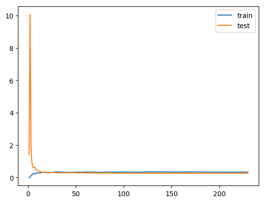
for i in range(10, len(train_data)+1, 10):
lin_reg = LinearRegression()
lin_reg.fit(train_data[:i], train_target[:i])
# LinearRegression().fit(X_train[:i], y_train[:i])
# 查看模型的预测情况:两种,模型基于训练数据集预测的情况(可以理解为模型拟合训练数据集的情况),模型基于测试数据集预测的情况
# 此处使用 lin_reg.predict(X_train[:i]),为训练模型的全部数据集
y_train_predict = lin_reg.predict(train_data[:i])
train_score.append(mean_squared_error(train_target[:i], y_train_predict))
y_test_predict = lin_reg.predict(test_data)
test_score.append(mean_squared_error(test_target, y_test_predict))
# np.sqrt(train_score):将列表 train_score 中的数开平方
plt.plot([i for i in range(1, len(train_score)+1)], train_score, label='train')
plt.plot([i for i in range(1, len(test_score)+1)], test_score, label='test')
# plt.legend():显示图例(如图形的 label);
plt.legend()
plt.show()
LinearRegression: 0.2642337917628173
定义绘制模型学习曲线函数
def plot_learning_curve(estimator, title, X, y, ylim=None, cv=None,
                        n_jobs=1, train_sizes=np.linspace(.1, 1.0, 5)):
    plt.figure()
    plt.title(title)
    if ylim is not None:
        plt.ylim(*ylim)
    plt.xlabel("Training examples")
    plt.ylabel("Score")
    train_sizes, train_scores, test_scores = learning_curve(
        estimator, X, y, cv=cv, n_jobs=n_jobs, train_sizes=train_sizes)
    train_scores_mean = np.mean(train_scores, axis=1)
    train_scores_std = np.std(train_scores, axis=1)
    test_scores_mean = np.mean(test_scores, axis=1)
    test_scores_std = np.std(test_scores, axis=1)

    print(train_scores_mean)
    print(test_scores_mean)

    plt.grid()

    plt.fill_between(train_sizes, train_scores_mean - train_scores_std,
                     train_scores_mean + train_scores_std, alpha=0.1,
                     color="r")
    plt.fill_between(train_sizes, test_scores_mean - test_scores_std,
                     test_scores_mean + test_scores_std, alpha=0.1, color="g")
    plt.plot(train_sizes, train_scores_mean, 'o-', color="r",
             label="Training score")
    plt.plot(train_sizes, test_scores_mean, 'o-', color="g",
             label="Cross-validation score")

    plt.legend(loc="best")
    return plt
def plot_learning_curve_old(algo, X_train, X_test, y_train, y_test):
    """绘制学习曲线:只需要传入算法(或实例对象)、X_train、X_test、y_train、y_test"""
    """当使用该函数时传入算法,该算法的变量要进行实例化,如:PolynomialRegression(degree=2),变量 degree 要进行实例化"""
    train_score = []
    test_score = []
    for i in range(10, len(X_train)+1, 10):
        algo.fit(X_train[:i], y_train[:i])

        y_train_predict = algo.predict(X_train[:i])
        train_score.append(mean_squared_error(y_train[:i], y_train_predict))

        y_test_predict = algo.predict(X_test)
        test_score.append(mean_squared_error(y_test, y_test_predict))

    plt.plot([i for i in range(1, len(train_score)+1)],
            train_score, label="train")
    plt.plot([i for i in range(1, len(test_score)+1)],
            test_score, label="test")

    plt.legend()
    plt.show()
# plot_learning_curve_old(LinearRegression(), train_data, test_data, train_target, test_target)
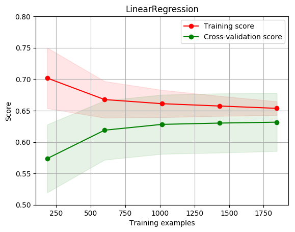
# 线性回归模型学习曲线
X = train_data.values
y = train_target.values

# 图一
title = r"LinearRegression"
cv = ShuffleSplit(n_splits=100, test_size=0.2, random_state=0)
estimator = LinearRegression()    #建模
plot_learning_curve(estimator, title, X, y, ylim=(0.5, 0.8), cv=cv, n_jobs=1)
[0.70183463 0.66761103 0.66101945 0.65732898 0.65360375]
[0.57364886 0.61882339 0.62809368 0.63012866 0.63158596]


<module 'matplotlib.pyplot' from '/opt/conda/envs/python35-paddle120-env/lib/python3.7/site-packages/matplotlib/pyplot.py'>
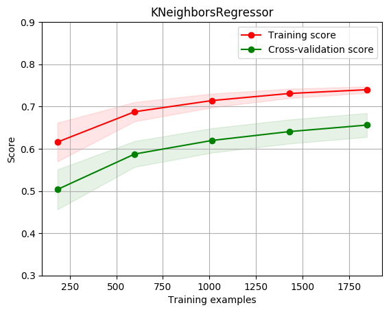
3.1.2 KNN近邻回归
for i in range(3,10):
    clf = KNeighborsRegressor(n_neighbors=i) # 最近三个
    clf.fit(train_data, train_target)
    score = mean_squared_error(test_target, clf.predict(test_data))
    print("KNeighborsRegressor:   ", score)
KNeighborsRegressor:    0.27619208861976163
KNeighborsRegressor:    0.2597627823313149
KNeighborsRegressor:    0.2628212724567474
KNeighborsRegressor:    0.26670982271241833
KNeighborsRegressor:    0.2659603905091448
KNeighborsRegressor:    0.26353694644788067
KNeighborsRegressor:    0.2673470579477979
# plot_learning_curve_old(KNeighborsRegressor(n_neighbors=5) , train_data, test_data, train_target, test_target)
# 绘制K近邻回归学习曲线
X = train_data.values
y = train_target.values

# K近邻回归
title = r"KNeighborsRegressor"
cv = ShuffleSplit(n_splits=100, test_size=0.2, random_state=0)

estimator = KNeighborsRegressor(n_neighbors=8)    #建模
plot_learning_curve(estimator, title, X, y, ylim=(0.3, 0.9), cv=cv, n_jobs=1)
[0.61581146 0.68763995 0.71414969 0.73084172 0.73976273]
[0.50369207 0.58753672 0.61969929 0.64062459 0.6560054 ]


<module 'matplotlib.pyplot' from '/opt/conda/envs/python35-paddle120-env/lib/python3.7/site-packages/matplotlib/pyplot.py'>
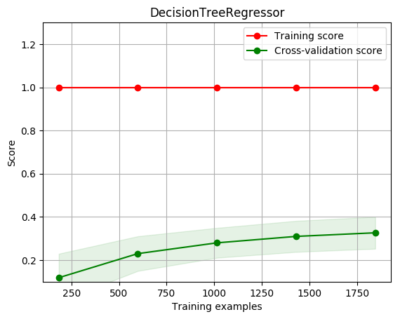
3.1.3决策树回归
clf = DecisionTreeRegressor()
clf.fit(train_data, train_target)
score = mean_squared_error(test_target, clf.predict(test_data))
print("DecisionTreeRegressor:   ", score)
DecisionTreeRegressor: 0.6405298823529413
# plot_learning_curve_old(DecisionTreeRegressor(), train_data, test_data, train_target, test_target)
X = train_data.values
y = train_target.values

# 决策树回归
title = r"DecisionTreeRegressor"
cv = ShuffleSplit(n_splits=100, test_size=0.2, random_state=0)

estimator = DecisionTreeRegressor()    #建模
plot_learning_curve(estimator, title, X, y, ylim=(0.1, 1.3), cv=cv, n_jobs=1)
[1. 1. 1. 1. 1.]
[0.11833987 0.22982731 0.2797608  0.30950084 0.32628853]


<module 'matplotlib.pyplot' from '/opt/conda/envs/python35-paddle120-env/lib/python3.7/site-packages/matplotlib/pyplot.py'>
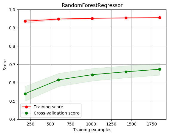
3.1.4 随机森林回归
clf = RandomForestRegressor(n_estimators=200) # 200棵树模型
clf.fit(train_data, train_target)
score = mean_squared_error(test_target, clf.predict(test_data))
print("RandomForestRegressor:   ", score)
# plot_learning_curve_old(RandomForestRegressor(n_estimators=200), train_data, test_data, train_target, test_target)
RandomForestRegressor: 0.24087959640588236
X = train_data.values
y = train_target.values

# 随机森林
title = r"RandomForestRegressor"
cv = ShuffleSplit(n_splits=100, test_size=0.2, random_state=0)

estimator = RandomForestRegressor(n_estimators=200)    #建模
plot_learning_curve(estimator, title, X, y, ylim=(0.4, 1.0), cv=cv, n_jobs=1)
[0.93619796 0.94798334 0.95197393 0.95415054 0.95570763]
[0.53953995 0.61531165 0.64366926 0.65941678 0.67319725]


<module 'matplotlib.pyplot' from '/opt/conda/envs/python35-paddle120-env/lib/python3.7/site-packages/matplotlib/pyplot.py'>
3.1.5 Gradient Boosting
from sklearn.ensemble import GradientBoostingRegressor

myGBR = GradientBoostingRegressor(alpha=0.9, criterion='friedman_mse', init=None,
                                  learning_rate=0.03, loss='huber', max_depth=14,
                                  max_features='sqrt', max_leaf_nodes=None,
                                  min_impurity_decrease=0.0, min_impurity_split=None,
                                  min_samples_leaf=10, min_samples_split=40,
                                  min_weight_fraction_leaf=0.0, n_estimators=10,
                                  warm_start=False)
# 参数已删除 presort=True, random_state=10, subsample=0.8, verbose=0,

myGBR.fit(train_data, train_target)
score = mean_squared_error(test_target, clf.predict(test_data))
print("GradientBoostingRegressor:   ", score)


myGBR = GradientBoostingRegressor(alpha=0.9, criterion='friedman_mse', init=None,
                                  learning_rate=0.03, loss='huber', max_depth=14,
                                  max_features='sqrt', max_leaf_nodes=None,
                                  min_impurity_decrease=0.0, min_impurity_split=None,
                                  min_samples_leaf=10, min_samples_split=40,
                                  min_weight_fraction_leaf=0.0, n_estimators=10,
                                  warm_start=False)
#为了快速展示n_estimators设置较小,实战中请按需设置

# plot_learning_curve_old(myGBR, train_data, test_data, train_target, test_target)
GradientBoostingRegressor: 0.906640574789251
X = train_data.values
y = train_target.values

# GradientBoosting
title = r"GradientBoostingRegressor"
cv = ShuffleSplit(n_splits=10, test_size=0.2, random_state=0)

estimator = GradientBoostingRegressor(alpha=0.9, criterion='friedman_mse', init=None,
                                  learning_rate=0.03, loss='huber', max_depth=14,
                                  max_features='sqrt', max_leaf_nodes=None,
                                  min_impurity_decrease=0.0, min_impurity_split=None,
                                  min_samples_leaf=10, min_samples_split=40,
                                  min_weight_fraction_leaf=0.0, n_estimators=10,
                                  warm_start=False)  #建模

plot_learning_curve(estimator, title, X, y, ylim=(0.4, 1.0), cv=cv, n_jobs=1)

#为了快速展示n_estimators设置较小,实战中请按需设置
3.1.6 lightgbm回归
# lgb回归模型
clf = lgb.LGBMRegressor(
        learning_rate=0.01,
        max_depth=-1,
        n_estimators=10,
        boosting_type='gbdt',
        random_state=2019,
        objective='regression',
    )
# #为了快速展示n_estimators设置较小,实战中请按需设置
# 训练模型
clf.fit(
        X=train_data, y=train_target,
        eval_metric='MSE',
        verbose=50
    )

score = mean_squared_error(test_target, clf.predict(test_data))
print("lightGbm:   ", score)
lightGbm: 0.906640574789251
X = train_data.values
y = train_target.values

# LGBM
title = r"LGBMRegressor"
cv = ShuffleSplit(n_splits=10, test_size=0.2, random_state=0)

estimator = lgb.LGBMRegressor(
    learning_rate=0.01,
    max_depth=-1,
    n_estimators=10,
    boosting_type='gbdt',
    random_state=2019,
    objective='regression'
    )    #建模

plot_learning_curve(estimator, title, X, y, ylim=(0.4, 1.0), cv=cv, n_jobs=1)

#为了快速展示n_estimators设置较小,实战中请按需设置
4.篇中总结
在工业蒸汽量预测上篇中,主要讲解了数据探索性分析:查看变量间相关性以及找出关键变量;数据特征工程对数据精进:异常值处理、归一化处理以及特征降维;在进行归回模型训练涉及主流ML模型:决策树、随机森林,lightgbm等。下一篇中将着重讲解模型验证、特征优化、模型融合等。
原项目链接:https://www.heywhale.com/home/column/64141d6b1c8c8b518ba97dcc


![一幅图像为f=[1 4 7;2 5 8;3 6 9],设kx=1.8,ky=1.3,试采用最邻近插值对其进行放大,写出新图像矩阵。](https://img2020.cnblogs.com/blog/2240937/202109/2240937-20210927141748825-1235120041.png)