分类算法之逻辑回归
逻辑回归(Logistic Regression),简称LR。它的特点是能够是我们的特征输入集合转化为0和1这两类的概率。一般来说,回归不用在分类问题上,因为回归是连续型模型,而且受噪声影响比较大。如果非要应用进入,可以使用逻辑回归。了解过线性回归之后再来看逻辑回归可以更好的理解。
优点:计算代价不高,易于理解和实现
缺点:容易欠拟合,分类精度不高
适用数据:数值型和标称型
逻辑回归
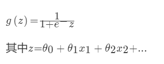
对于回归问题后面会介绍,Logistic回归本质上是线性回归,只是在特征到结果的映射中加入了一层函数映射,即先把特征线性求和,然后使用函数g(z)将最为假设函数来预测。g(z)可以将连续值映射到0和1上。Logistic回归用来分类0/1问题,也就是预测结果属于0或者1的二值分类问题
映射函数为:
映射出来的效果如下如:

sklearn.linear_model.LogisticRegression
逻辑回归类
class sklearn.linear_model.LogisticRegression(penalty='l2', dual=False, tol=0.0001, C=1.0, fit_intercept=True, intercept_scaling=1, class_weight=None, random_state=None, solver='liblinear', max_iter=100, multi_class='ovr', verbose=0, warm_start=False, n_jobs=1)
  """
  :param C: float,默认值:1.0

  :param penalty: 特征选择的方式

  :param tol: 公差停止标准
  """

from sklearn.model_selection import train_test_split
from sklearn.datasets import load_digits
from sklearn.linear_model import LogisticRegression
LR = LogisticRegression(C=1.0, penalty='l1', tol=0.01)
X_train, X_test, y_train, y_test = train_test_split(X, y, test_size=0.33, random_state=42)
LR.fit(X_train,y_train)
LR.predict(X_test)
LR.score(X_test,y_test)
0.96464646464646464
# c=100.0
0.96801346801346799
属性
coef_
决策功能的特征系数
Cs_
数组C,即用于交叉验证的正则化参数值的倒数
特点分析
线性分类器可以说是最为基本和常用的机器学习模型。尽管其受限于数据特征与分类目标之间的线性假设,我们仍然可以在科学研究与工程实践中把线性分类器的表现性能作为基准。
恶性良性肿瘤预测
# 导入模块
from sklearn.linear_model import LogisticRegression #逻辑回归
from sklearn.preprocessing import StandardScaler #标准化
from sklearn.metrics import classification_report # 召回率
from sklearn.model_selection import train_test_split # 数据分割
import pandas as pd
import numpy as np
import matplotlib.pyplot as plt
# 创建特征名列表
feature_names = ["Sample code number", "Clump Thickness",
                 "Uniformity of Cell Size", "Uniformity of Cell Shape", "Marginal Adhesion", "Single Epithelial Cell Size", "Bare Nuclei", "Bland Chromatin", "Normal Nucleoli", "Mitoses", "Class"]
# 读取数据
data = pd.read_csv("./breast-cancer-wisconsin.data", names=feature_names)
data.info()
<class 'pandas.core.frame.DataFrame'>
RangeIndex: 699 entries, 0 to 698
Data columns (total 11 columns):
 #   Column                       Non-Null Count  Dtype
---  ------                       --------------  -----
 0   Sample code number           699 non-null    int64
 1   Clump Thickness              699 non-null    int64
 2   Uniformity of Cell Size      699 non-null    int64
 3   Uniformity of Cell Shape     699 non-null    int64
 4   Marginal Adhesion            699 non-null    int64
 5   Single Epithelial Cell Size  699 non-null    int64
 6   Bare Nuclei                  699 non-null    object
 7   Bland Chromatin              699 non-null    int64
 8   Normal Nucleoli              699 non-null    int64
 9   Mitoses                      699 non-null    int64
 10  Class                        699 non-null    int64
dtypes: int64(10), object(1)
memory usage: 60.2+ KB
# 数据处理
# 将所有?更改成nan
data = data.replace(to_replace="?", value=np.nan)
# 将 Bare Nuclei 类型转换成float类型
data["Bare Nuclei"] = data["Bare Nuclei"].astype("float")
# 将所有nan填充成他所在列的均值
data = data.fillna(data.mean())
# 查看是否还有NAN
data.isna().sum()
Sample code number             0
Clump Thickness                0
Uniformity of Cell Size        0
Uniformity of Cell Shape       0
Marginal Adhesion              0
Single Epithelial Cell Size    0
Bare Nuclei                    0
Bland Chromatin                0
Normal Nucleoli                0
Mitoses                        0
Class                          0
dtype: int64
# 数据标准化
x_train, x_test, y_train, y_test = train_test_split(data.iloc[:,1:10], data.loc[:,"Class"])
# 数据标准化
std = StandardScaler().fit(x_train)
x_train = std.transform(x_train)
x_test = std.transform(x_test)
# 逻辑回归预测肿瘤
# 实例化param:c 正则化力度,penalty 正则化方式
log = LogisticRegression(penalty="l2",C=1)
# 训练测试集和训练集
log.fit(x_train, y_train)
LogisticRegression(C=1)
In a Jupyter environment, please rerun this cell to show the HTML representation or trust the notebook.
On GitHub, the HTML representation is unable to render, please try loading this page with nbviewer.org.
LogisticRegression(C=1)
# 查看预测得分
score = log.score(x_test, y_test)
score
0.9542857142857143
# 查看预测的结果
y_predict = log.predict(x_test)
y_predict
array([2, 2, 2, 4, 2, 2, 2, 2, 2, 2, 2, 4, 2, 2, 4, 2, 4, 2, 2, 2, 2, 2,
       2, 2, 2, 2, 4, 2, 2, 2, 2, 2, 2, 2, 4, 2, 4, 4, 2, 4, 2, 4, 2, 2,
       2, 2, 4, 4, 4, 2, 2, 4, 2, 2, 4, 4, 2, 4, 2, 2, 2, 2, 2, 2, 2, 2,
       2, 2, 2, 4, 2, 2, 4, 4, 2, 2, 4, 2, 2, 2, 2, 2, 4, 2, 4, 2, 2, 2,
       2, 2, 2, 2, 2, 4, 2, 4, 2, 4, 2, 2, 2, 4, 4, 2, 2, 2, 2, 4, 2, 4,
       2, 2, 2, 2, 4, 4, 4, 2, 2, 2, 4, 4, 2, 4, 4, 2, 2, 4, 2, 2, 2, 4,
       2, 2, 2, 4, 2, 4, 2, 2, 2, 2, 4, 2, 2, 2, 4, 4, 2, 4, 2, 2, 4, 4,
       2, 4, 2, 4, 2, 2, 2, 2, 4, 2, 2, 2, 2, 2, 4, 4, 4, 2, 2, 2, 2],
      dtype=int64)
# 查看回归系数
log.coef_
array([[ 1.5859245 , -0.1730868 ,  0.79379743,  1.02638845,  0.00220408,
         1.44509346,  1.03614595,  0.6169744 ,  1.10281087]])
# 查看召回率
recall = classification_report(y_test, log.predict(x_test),labels=[2,4], target_names=["良性肿瘤","恶性肿瘤"])
print(recall)
              precision    recall  f1-score   support

        良性肿瘤       0.98      0.96      0.97       124
        恶性肿瘤       0.91      0.94      0.92        51

    accuracy                           0.95       175
   macro avg       0.94      0.95      0.95       175
weighted avg       0.96      0.95      0.95       175
非监督学习之k-means
K-means通常被称为劳埃德算法,这在数据聚类中是最经典的,也是相对容易理解的模型。算法执行的过程分为4个阶段。
- 1.首先,随机设K个特征空间内的点作为初始的聚类中心。
- 2.然后,对于根据每个数据的特征向量,从K个聚类中心中寻找距离最近的一个,并且把该数据标记为这个聚类中心。
- 3.接着,在所有的数据都被标记过聚类中心之后,根据这些数据新分配的类簇,通过取分配给每个先前质心的所有样本的平均值来创建新的质心重,新对K个聚类中心做计算。
- 4.最后,计算旧和新质心之间的差异,如果所有的数据点从属的聚类中心与上一次的分配的类簇没有变化,那么迭代就可以停止,否则回到步骤2继续循环。
K均值等于具有小的全对称协方差矩阵的期望最大化算法
sklearn.cluster.KMeans
class sklearn.cluster.KMeans(n_clusters=8, init='k-means++', n_init=10, max_iter=300, tol=0.0001, precompute_distances='auto', verbose=0, random_state=None, copy_x=True, n_jobs=1, algorithm='auto')
  """
  :param n_clusters:要形成的聚类数以及生成的质心数

  :param init:初始化方法,默认为'k-means ++',以智能方式选择k-均值聚类的初始聚类中心,以加速收敛;random,从初始质心数据中随机选择k个观察值(行

  :param n_init:int,默认值:10使用不同质心种子运行k-means算法的时间。最终结果将是n_init连续运行在惯性方面的最佳输出。

  :param n_jobs:int用于计算的作业数量。这可以通过并行计算每个运行的n_init。如果-1使用所有CPU。如果给出1,则不使用任何并行计算代码,这对调试很有用。对于-1以下的n_jobs,使用(n_cpus + 1 + n_jobs)。因此,对于n_jobs = -2,所有CPU都使用一个。

  :param random_state:随机数种子,默认为全局numpy随机数生成器
  """
from sklearn.cluster import KMeans
import numpy as np
X = np.array([[1, 2], [1, 4], [1, 0],[4, 2], [4, 4], [4, 0]])
kmeans = KMeans(n_clusters=2, random_state=0)
方法
fit(X,y=None)
使用X作为训练数据拟合模型
kmeans.fit(X)
predict(X)
预测新的数据所在的类别
kmeans.predict([[0, 0], [4, 4]])
array([0, 1], dtype=int32)
属性
cluster*centers*
集群中心的点坐标
kmeans.cluster_centers_
array([[ 1.,  2.],
       [ 4.,  2.]])
labels_
每个点的类别
kmeans.labels_
用户类型聚类
# 导入模块
import pandas as pd
from sklearn.cluster import KMeans #聚类算法
from sklearn.decomposition import PCA # 数据降维
# products.csv                               商品信息
# order_products__prior.csv                 订单与商品信息
# orders.csv                                   用户的订单信息
# aisles.csv                                    商品所属具体物品类别
# 读取数据
products = pd.read_csv("../data/products.csv")
order_products__prior = pd.read_csv("../data/order_products__prior.csv")
orders = pd.read_csv("../data/orders.csv")
aisles = pd.read_csv("../data/aisles.csv")
products.columns
Index(['product_id', 'product_name', 'aisle_id', 'department_id'], dtype='object')
order_products__prior.columns
Index(['order_id', 'product_id', 'add_to_cart_order', 'reordered'], dtype='object')
orders.columns
Index(['order_id', 'user_id', 'eval_set', 'order_number', 'order_dow',
       'order_hour_of_day', 'days_since_prior_order'],
      dtype='object')
aisles.columns
Index(['aisle_id', 'aisle'], dtype='object')
data = pd.merge(products, order_products__prior, on=["product_id","product_id"])
data = pd.merge(data, orders, on=["order_id", "order_id"])
data = pd.merge(data, aisles, on=["aisle_id", "aisle_id"])
data.head()
| product_id | product_name | aisle_id | department_id | order_id | add_to_cart_order | reordered | user_id | eval_set | order_number | order_dow | order_hour_of_day | days_since_prior_order | aisle | |
|---|---|---|---|---|---|---|---|---|---|---|---|---|---|---|
| 0 | 1 | Chocolate Sandwich Cookies | 61 | 19 | 1107 | 7 | 0 | 38259 | prior | 2 | 1 | 11 | 7.0 | cookies cakes |
| 1 | 1 | Chocolate Sandwich Cookies | 61 | 19 | 5319 | 3 | 1 | 196224 | prior | 65 | 1 | 14 | 1.0 | cookies cakes |
| 2 | 1 | Chocolate Sandwich Cookies | 61 | 19 | 7540 | 4 | 1 | 138499 | prior | 8 | 0 | 14 | 7.0 | cookies cakes |
| 3 | 1 | Chocolate Sandwich Cookies | 61 | 19 | 9228 | 2 | 0 | 79603 | prior | 2 | 2 | 10 | 30.0 | cookies cakes |
| 4 | 1 | Chocolate Sandwich Cookies | 61 | 19 | 9273 | 30 | 0 | 50005 | prior | 1 | 1 | 15 | NaN | cookies cakes |
# 交叉表
corss = pd.crosstab(data["user_id"], data["aisle"])
corss
| aisle | air fresheners candles | asian foods | baby accessories | baby bath body care | baby food formula | bakery desserts | baking ingredients | baking supplies decor | beauty | beers coolers | ... | spreads | tea | tofu meat alternatives | tortillas flat bread | trail mix snack mix | trash bags liners | vitamins supplements | water seltzer sparkling water | white wines | yogurt |
|---|---|---|---|---|---|---|---|---|---|---|---|---|---|---|---|---|---|---|---|---|---|
| user_id | |||||||||||||||||||||
| 1 | 0 | 0 | 0 | 0 | 0 | 0 | 0 | 0 | 0 | 0 | ... | 1 | 0 | 0 | 0 | 0 | 0 | 0 | 0 | 0 | 1 |
| 2 | 0 | 3 | 0 | 0 | 0 | 0 | 2 | 0 | 0 | 0 | ... | 3 | 1 | 1 | 0 | 0 | 0 | 0 | 2 | 0 | 42 |
| 3 | 0 | 0 | 0 | 0 | 0 | 0 | 0 | 0 | 0 | 0 | ... | 4 | 1 | 0 | 0 | 0 | 0 | 0 | 2 | 0 | 0 |
| 4 | 0 | 0 | 0 | 0 | 0 | 0 | 0 | 0 | 0 | 0 | ... | 0 | 0 | 0 | 1 | 0 | 0 | 0 | 1 | 0 | 0 |
| 5 | 0 | 2 | 0 | 0 | 0 | 0 | 0 | 0 | 0 | 0 | ... | 0 | 0 | 0 | 0 | 0 | 0 | 0 | 0 | 0 | 3 |
| ... | ... | ... | ... | ... | ... | ... | ... | ... | ... | ... | ... | ... | ... | ... | ... | ... | ... | ... | ... | ... | ... |
| 206205 | 0 | 0 | 1 | 0 | 0 | 0 | 0 | 0 | 0 | 0 | ... | 0 | 0 | 0 | 0 | 0 | 0 | 0 | 0 | 0 | 5 |
| 206206 | 0 | 4 | 0 | 0 | 0 | 0 | 4 | 1 | 0 | 0 | ... | 1 | 0 | 0 | 0 | 0 | 1 | 0 | 1 | 0 | 0 |
| 206207 | 0 | 0 | 0 | 0 | 1 | 0 | 0 | 0 | 0 | 0 | ... | 3 | 4 | 0 | 2 | 1 | 0 | 0 | 11 | 0 | 15 |
| 206208 | 0 | 3 | 0 | 0 | 3 | 0 | 4 | 0 | 0 | 0 | ... | 5 | 0 | 0 | 7 | 0 | 0 | 0 | 0 | 0 | 33 |
| 206209 | 0 | 1 | 0 | 0 | 0 | 0 | 0 | 0 | 0 | 0 | ... | 0 | 0 | 0 | 0 | 0 | 1 | 0 | 0 | 0 | 3 |
206209 rows × 134 columns
# 数据降维
pca = PCA(n_components=0.9)
data_pca = pca.fit_transform(corss)
data_pca
array([[-2.42156587e+01,  2.42942720e+00, -2.46636975e+00, ...,
         6.86800336e-01,  1.69439402e+00, -2.34323022e+00],
       [ 6.46320807e+00,  3.67511165e+01,  8.38255336e+00, ...,
         4.12121252e+00,  2.44689740e+00, -4.28348478e+00],
       [-7.99030162e+00,  2.40438257e+00, -1.10300641e+01, ...,
         1.77534453e+00, -4.44194030e-01,  7.86665571e-01],
       ...,
       [ 8.61143331e+00,  7.70129866e+00,  7.95240226e+00, ...,
        -2.74252456e+00,  1.07112531e+00, -6.31925661e-02],
       [ 8.40862199e+01,  2.04187340e+01,  8.05410372e+00, ...,
         7.27554259e-01,  3.51339470e+00, -1.79079914e+01],
       [-1.39534562e+01,  6.64621821e+00, -5.23030367e+00, ...,
         8.25329076e-01,  1.38230701e+00, -2.41942061e+00]])
# 实例化Kmeans
km = KMeans(n_clusters=4)
# 训练数据
km.fit(data_pca)
D:\DeveloperTools\Anaconda\lib\site-packages\sklearn\cluster\_kmeans.py:870: FutureWarning: The default value of `n_init` will change from 10 to 'auto' in 1.4. Set the value of `n_init` explicitly to suppress the warning
  warnings.warn(
KMeans(n_clusters=4)
In a Jupyter environment, please rerun this cell to show the HTML representation or trust the notebook.
On GitHub, the HTML representation is unable to render, please try loading this page with nbviewer.org.
KMeans(n_clusters=4)
# 查看聚合结果
km_preduct = km.predict(data_pca)
km_preduct
array([0, 3, 0, ..., 3, 1, 0])
# 显示聚类的结果
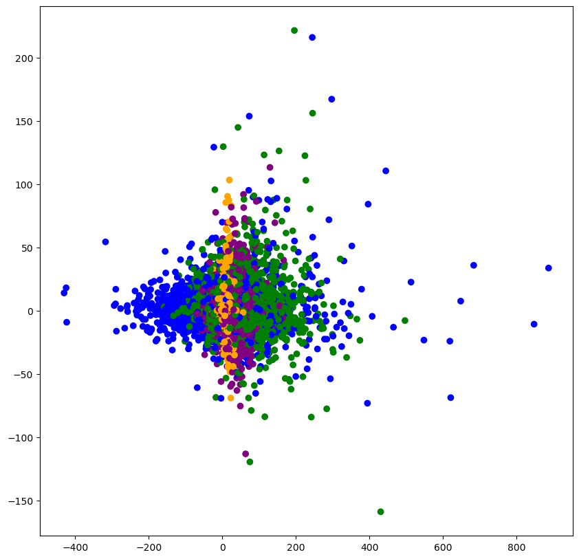
plt.figure(figsize=(10,10))
colored = ['orange', 'green', 'blue', 'purple']
colr = [colored[i] for i in km_preduct]
plt.scatter(data_pca[:, 1], data_pca[:, 20], color=colr)
plt.show()