1. Anomaly Detection

I'd like to tell you about a problem called Anomaly Detection. This is a reasonably commonly usetype machine learning. And one of the interesting aspects is that it's mainly for unsupervised problem, that there's some aspects of it that are also very similar to sort of the supervised learning problem.

1.1 Algorithm

Training set: \(x^{(1)},...,x^{(m)}\), each example is \(x \in \mathbb{R}^n\).
Chose features \(x_j\) that you think might be indicative of anlmalous examples.
Choose features that might take on unusually large or small values in the event of an anomaly.
Fit prarmeters \(\mu_1,..., \mu_n, \sigma^2_i,...,\sigma^2_n\)
\(x_1 \sim N(\mu_1 , \sigma^2_1)\), \(x_2 \sim N(\mu_2 , \sigma^2_2)\),...,\(x_n \sim N(\mu_n , \sigma^2_n)\)
\(\mu_j = \frac{1}{m} \sum_{i=1}^{m}x_{j}^{(i)}\)
\(\sigma^2_j = \frac{1}{m} \sum_{i=1}^{m}(x_{j}^{(i)}-\mu_j)^2\)
Given new example \(x\), compute \(p(x)\):
\(\begin{align*}
P(x) &= P(x_1;\mu_1 , \sigma^2_1)P(x_2;\mu_2 , \sigma^2_2) \cdots P(x_n;\mu_n , \sigma^2_n)\\
&=\prod_{j=1}^{n} P(x_j;\mu_j , \sigma^2_j) \\
&=\prod_{j=1}^{n} \frac{1} {{\sigma_j \sqrt{2\pi}}}exp(-\frac{(x_j -\mu_j)^2}{2\sigma^2_j})
\end{align*}\)
Anomaly if \(p(x)< \epsilon\)

但是怎么选择 \(\epsilon\) 呢？这就得用到实际的标签了。这就是说为什么它既是无监督学习，也有一点监督学习的味道。

1.2 Developing and evaluating an anomaly detection system.

When developing a learning algorithm (choosing features, etc.), making decisions is much easier if we have a way of evaluating our learning algorithm.

Assume we have some labeled data, of anomalous and non-anomalous examples. (\(y=0\) if normal, \(y=1\) if anomalous).

Training set: \(x^{(1)},...,x^{(m)}\) assume normal examples/not anomalous)

In anomaly detection, we fit a model \(p(x)\) to a set of negative \((y=0)\) examples, without using any positive examples we may have collected of previously observed anomalies.We want to model "normal" examples, so we only use negative examples \((y=0)\;normal\) in training.

Cross validation set: \((x^{(1)}_{cv},y^{(1)}_{cv}), (x^{(2)}_{cv},y^{(2)}_{cv}), ..., (x^{(m)}_{cv},y^{(m)}_{cv})\)

Test set： \((x^{(1)}_{test},y^{(1)}_{test}), (x^{(2)}_{test},y^{(2)}_{test}), ..., (x^{(m)}_{test},y^{(m)}_{test})\)

1.2.1 For an Aircraft engines motivating example:

10000 good(normal) engines
20 flawed engines(anomalous)

Training set: 6000 good engines
CV: 2000 good engines (\(y=0\)), 10 anomalous (\(y=1\))
Test: 2000 good engines (\(y=0\)), 10 anomalous (\(y=1\))

Fit model \(p(x)\) on training set \(x^{(1)},...,x^{(m)}\)
On a cross validation/test example \(x\), predict

\[y=\left\{\begin{matrix}
1 \; if \; p(x) < \epsilon \; \text{anomaly}\\
0 \; if \; p(x) \geq \epsilon \; \text{normal}\\
\end{matrix}\right.
\]

Give an parameter \(\epsilon\), find metrics:

True positive, false positive, false negative, true negative.
Rrecision/Recall
F1-score

对于一系列的 \(\epsilon\)，选择最大值的F1-score

\[prec \; = \frac{tp}{tp+fp}\\
rec \; = \frac{tp}{tp+fn}\\
F_1 \; = \frac{2 \cdot prec \cdot rec}{prec+rec}
\]

where

\(tp\) is the number of true positives: the ground truth label says it’s an
anomaly and our algorithm correctly classified it as an anomaly.
\(fp\) is the number of false positives: the ground truth label says it’s not
an anomaly, but our algorithm incorrectly classified it as an anomaly.
\(fn\) is the number of false negatives: the ground truth label says it’s an
anomaly, but our algorithm incorrectly classified it as not being anomalous.

tp = sum((predictions==1) & (yval==1));
fp = sum((predictions==1) & (yval==0));
fn = sum((predictions==0) & (yval==1));

1.3 Anomaly detection vs. supervised learning

Anomaly detection	Supervised Learning
Very small number of positive examples \((y=1)\). ( 0-20 or 0-50 is common). Large number of negative \((y=0)\)examples.	Large number of positive and negative examples.
Many different “types” of anomalies. Hard for any algorithm to learn from positive examples what the anomalies look like; future anomalies may look nothing like any of the anomalous examples we've seen so far.	Enough posi-ve examples for algorithm to get a sense of what positive examples are like, future positive examples likely to be similar to ones in training set.
Fraud detection	Email spam classification
Manufacturing(e.g. aircraft engines)	Weather prediction(sunny/rainy/tec)
Monitoring machines in a data center	Cancer classification

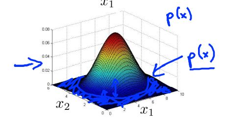
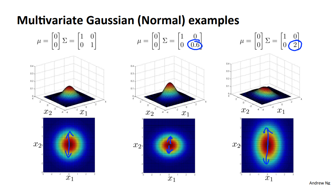
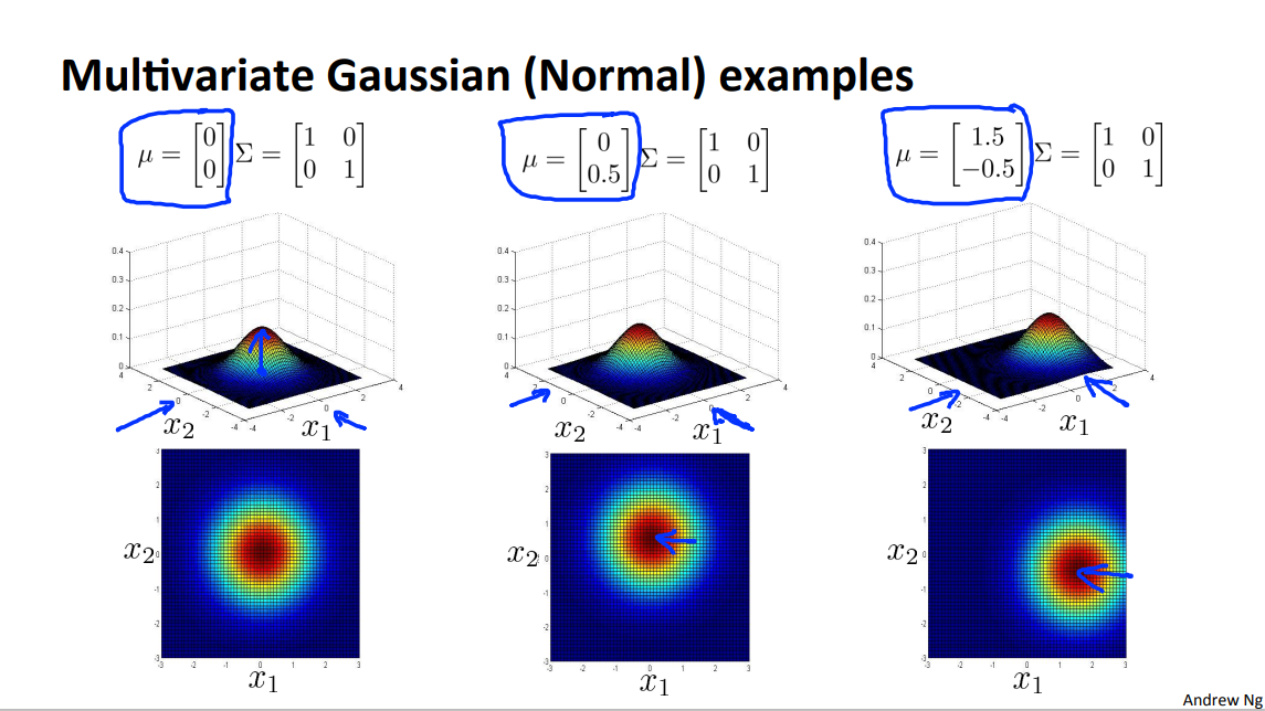
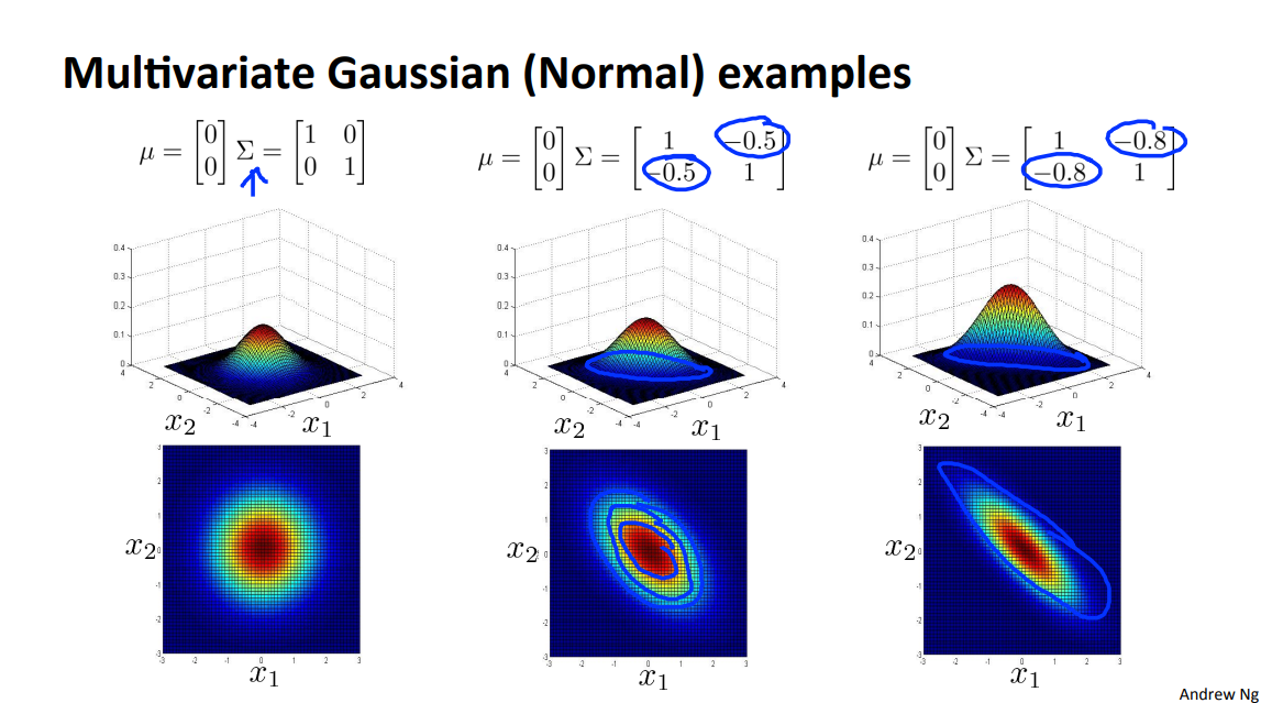
1.4 Multivariate Gaussian distribution

Machine Learning Week_9 Anomaly Detection and Recommend System-小白菜博客
这种斜方向的分布是普通的高斯分布拟合不出来的，所以就要用到 Multivariate Gaussian distribution。

1.4.1 Algorithm

Fit Model \(p(x)\) by setting
\(x^{(1)},...,x^{(m)}\)
\(\mu =\frac{1}{m} \sum_{i=1}^{m} x^{(i)}\)
\(\Sigma = \frac{1}{m} \sum_{i=1}^{m}(x^{(i)}-\mu)(x^{(i)}-\mu)^T\)
Given a new example \(x\), compute

\[p(x;\mu, \Sigma) = \frac{1} {|\Sigma|^{\frac{1}{2}} (2\pi)^{\frac{n}{2}}} exp(-\frac{1}{2}(x -\mu)^T \Sigma^{-1}(x-\mu))
\]

Flag an anomaly if \(p(x)< \epsilon\)

下面是一些图片，注意\(\Sigma\)矩阵的斜对角元素，以及正负。 形状会比普通的高斯分布多一点。普通高斯分布对应\(\Sigma\)矩阵的斜对角元素为0的情况。

Orginal Model

\(P(x) = P(x_1;\mu_1 , \sigma^2_1)P(x_2;\mu_2 , \sigma^2_2) \cdots P(x_n;\mu_n , \sigma^2_n)\)
Manually create features to capture anomalies where \(x_1,x_2\) take unusual combinations of
values.
Computationally cheaper ( alternatively, scales better to large n)
OK even if \(m\) training set size) is small

Multivariate Guassian

\(p(x;\mu, \Sigma) = \frac{1} {|\Sigma|^{\frac{1}{2}} (2\pi)^{\frac{n}{2}}} exp(-\frac{1}{2}(x -\mu)^T \Sigma^{-1}(x-\mu))\)
Automatically captures correlations between features
Computationally more expensive
Must have \(m>n\) , or else \(\Sigma\) is non-invertible.

2 Rcommender system

2.1 Problem Formulation

In this next set of videos, I would like to tell you about recommender systems. There are two reasons, I had two motivations for why I wanted to talk about recommender systems.

The first is just that it is an important application of machine learning. Over the last few years, occasionally I visit different, you know, technology companies here in Silicon Valley and I often talk to people working on machine learning applications there and so I've asked people what are the most important applications of machine learning or what are the machine learning applications that you would most like to get an improvement in the performance of. And one of the most frequent answers I heard was that there are many groups out in Silicon Valley now, trying to build better recommender systems.

So, if you think about what the websites are like Amazon, or what Netflix or what eBay, or what iTunes Genius, made by Apple does, there are many websites or systems that try to recommend new products to use. So, Amazon recommends new books to you, Netflix try to recommend new movies to you, and so on. And these sorts of recommender systems, that look at what books you may have purchased in the past, or what movies you have rated in the past, but these are the systems that are responsible for today, a substantial fraction of Amazon's revenue and for a company like Netflix, the recommendations that they make to the users is also responsible for a substantial fraction of the movies watched by their users. And so an improvement in performance of a recommender system can have a substantial and immediate impact on the bottom line of many of these companies.

Recommender systems is kind of a funny problem, within academic machine learning so that we could go to an academic machine learning conference, the problem of recommender systems, actually receives relatively little attention, or at least it's sort of a smaller fraction of what goes on within Academia. But if you look at what's happening, many technology companies, the ability to build these systems seems to be a high priority for many companies. And that's one of the reasons why I want to talk about them in this class.

The second reason that I want to talk about recommender systems is that as we approach the last few sets of videos of this class I wanted to talk about a few of the big ideas in machine learning and share with you, you know, some of the big ideas in machine learning. And we've already seen in this class that features are important for machine learning, the features you choose will have a big effect on the performance of your learning algorithm. So there's this big idea in machine learning, which is that for some problems, maybe not all problems, but some problems, there are** algorithms that can try to automatically learn a good set of features for you.** So rather than trying to hand design, or hand code the features, which is mostly what we've been doing so far, there are a few settings where you might be able to have an algorithm, just to learn what feature to use, and the recommender systems is just one example of that sort of setting. There are many others, but engraved through recommender systems, will be able to go a little bit into this idea of learning the features and you'll be able to see at least one example of this, I think, big idea in machine learning as well.

2.2

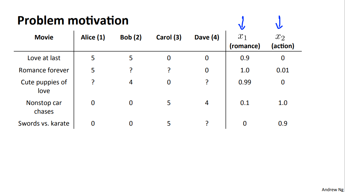
\(n_u\) = no.users
\(n_m\) = no.movies
\(r(i,j)\) = 1 if user j has rated movie i
\(y^{(i,j)}\) = rating given by user j to movie i (defined only if \(r(i,j)\) = 1)
\(\theta^{(j)}\) = parameter vector for user j
\(x^{(i)}\) = feature vector form movie i
For user j movie i, predicted rating:\((\theta^{(j)})^T(x^{(i)})\)

2.2.1 Optimization objective:

To learn \(\theta^{(j)}\) (parameter for user \(j\)):

\[min_{\theta^{(j)}} \frac{1}{2}\sum_{i:r(i,j)=1}\left ( (\theta^{(j)})^Tx^{(i)} -y^{(i,j)} \right )^2 + \frac{\lambda}{2}\sum_{k=1}^{n}(\theta^{(j)}_k)^2
\]

只用用户评价过的电影来计算代价函数，\(i:r(i,j)=1\), 但是在一个矩阵运算中，评没评过都一块算了，但是算完没评过的就得置0. 没评价过的就记为0了。同时对应的导数值也为0。设置为0之后, 相加，相减就不影响了。

To learn \(\theta^{(1)}\), \(\theta^{(2)}\),..., \(\theta^{(n_u)}\)

\[min_{\theta^{(j)},...,\theta^{(n_u)}} \frac{1}{2}\sum_{j=1}^{n_u} \sum_{i:r(i,j)=1}\left ( (\theta^{(j)})^Tx^{(i)} -y^{(i,j)} \right )^2 + \frac{\lambda}{2}\sum_{j=1}^{n_u} \sum_{k=1}^{n}(\theta^{(j)}_k)^2
\]

Given \(\theta^{(1)}\), \(\theta^{(2)}\),..., \(\theta^{(n_u)}\), To learn \(x^{(i)}\) (parameter for movie \(i\)):

\[min_{x^{(i)}} \frac{1}{2}\sum_{j:r(i,j)=1}\left ( (\theta^{(j)})^Tx^{(i)} -y^{(i,j)} \right )^2 + \frac{\lambda}{2}\sum_{k=1}^{n}(x^{(i)}_k)^2
\]

Given \(\theta^{(1)}\), \(\theta^{(2)}\),..., \(\theta^{(n_u)}\), To learn \(x^{(i)}\),...,\(x^{(n_m)}\) (parameter for movie \(i\)):

\[min_{x^{(1)},...,x^{(n_m)}} \frac{1}{2} \sum_{i=1}^{n_m} \sum_{j:r(i,j)=1}\left ( (\theta^{(j)})^Tx^{(i)} -y^{(i,j)} \right )^2 + \frac{\lambda}{2} \sum_{i=1}^{n_m} \sum_{k=1}^{n}(x^{(i)}_k)^2
\]

Collaborative filtering optimization objective

Minimizing \(\theta^{(1)}\), \(\theta^{(2)}\),..., \(\theta^{(n_u)}\) and \(x^{(i)}\),...,\(x^{(n_m)}\) simutaneously

\[min_{\theta^{(j)},...,\theta^{(n_u)},x^{(1)},...,x^{(n_m)}} = J(\theta^{(j)},...,\theta^{(n_u)},x^{(1)},...,x^{(n_m)})= \frac{1}{2} \sum_{(i,j):r(i,j)=1}\left ( (\theta^{(j)})^Tx^{(i)} -y^{(i,j)} \right )^2 +\frac{\lambda}{2}\sum_{j=1}^{n_u} \sum_{k=1}^{n}(\theta^{(j)}_k)^2+ \frac{\lambda}{2} \sum_{i=1}^{n_m} \sum_{k=1}^{n}(x^{(i)}_k)^2
\]

Collaborative filtering algorithm

Initialize \(\theta^{(1)}\), \(\theta^{(2)}\),..., \(\theta^{(n_u)}\), \(x^{(i)}\),...,\(x^{(n_m)}\) to small random values.
Minimize \(J(\theta^{(j)},...,\theta^{(n_u)},x^{(1)},...,x^{(n_m)})\) using gradient descent . (Linear regression)
For a user with parameters \(\theta\) and a movie with (learned) features x, predict a star rating of \(\theta^Tx\).

J = (1/2) * sum(sum(((X*Theta' - Y).^2) .* R)) + (lambda/2)*sum(sum(Theta.^2)) + (lambda/2)*sum(sum(X.^2));
X_grad = (Theta' * ((Theta * X' - Y').* R'))' + lambda * X;
Theta_grad = (X' * ((X * Theta' - Y).* R ))' + lambda * Theta;