KNN(K-NearestNeighbor)算法
KNN算法是有监督学习中的分类算法.
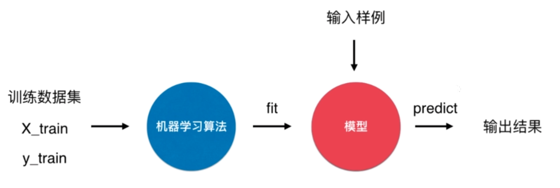
KNN算法很特殊,可以被认为是没有模型的算法,也可以认为其训练数据集就是模型本身。
KNN算法的原理
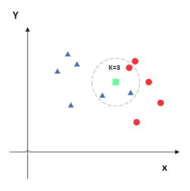
KNN的原理就是当预测一个新的值\(x\)的时候,根据它距离最近的\(K\)个点是什么类别来判断\(x\)属于哪个类别。
KNN算法的实现
实现knn算法需要计算两个点之前的距离,计算距离常用的有直线距离(欧拉距离)和曼哈顿距离。(这里使用欧拉距离来进行计算)
- 欧拉距离
\[\sqrt{(x^{(a)}_{(1)} - x^{(b)}_{(1)})^2 + \cdots + (x^{(a)}_{(n)} - x^{(b)}_{(n)})^2} = ({\sum _{i=1}^n(x_{(i)}^{(a)} - x_{(i)}^{(b)})^2})^{(\frac{1}{2})}
\]
\]
- 曼哈顿距离
\[\sum_{i=1}^n {|x_{(i)}^{(a)} - x_{(i)}^{(b)}|}
\]
\]
- 明可夫斯基距离
- \(p\)为超参数
- 默认值为\(2\)的时候取的为欧拉距离
\[(\sum_{i=1}^{n} |x_{(i)}^{(a)} - x_{(i)}^{(b)}|^{p})^{(\frac{1}{p})}
\]
\]
- 向量空间余弦相似度
一个向量空间中两个向量夹角间的余弦值作为衡量两个个体之间差异的大小,余弦值接近1,夹角趋于0,表明两个向量越相似,余弦值接近于0,夹角趋于90度,表明两个向量越不相似。
\[\cos \theta = \frac{\displaystyle\sum_{i=1}^n (x_{(i)}^{(a)}\times x_{(i)}^{(b)})}{\sqrt{\displaystyle\sum_{i=1}^{n} (x_{(i)}^{(a)})^2}\times \sqrt{\displaystyle\sum_{i=1}^{n}(x_{(i)}^{(b)})^{2}}}
\]
\]
- 皮尔森相关系数
两个变量之间的协方差和标准差的商
\[\rho _{X,Y} =
\frac{\mathrm{cov}(X,Y)}{\sigma_{X}\sigma_{Y}}
= \frac{E[(X-\mu_{x})(Y-\mu_{y})]}{\sigma_{X}\sigma_{Y}}
\frac{\mathrm{cov}(X,Y)}{\sigma_{X}\sigma_{Y}}
= \frac{E[(X-\mu_{x})(Y-\mu_{y})]}{\sigma_{X}\sigma_{Y}}
\]
import numpy as np
from math import sqrt
from collections import Counter


class KNN_Classifier:

    def __init__(self, k):
        # 初始化分类器
        assert k >= 1, "k must be valid"
        self.k = k
        self._x_train = None
        self._y_train = None

    def fit(self, x_train, y_train):
        # 根据训练集来训练
        assert x_train.shape[0] == y_train.shape[0], \
            "the size of x_train and y_train must be common"
        assert self.k <= x_train.shape[0], \
            "the size of train can't less than k"
        self._x_train = x_train
        self._y_train = y_train
        return self

    # 传入的需要预测的数据
    def predict(self, x_predict):
        assert self._x_train is not None and self._y_train is not None, \
            "must fit it before predict"
        assert x_predict.shape[1] == self._x_train.shape[1], \
            "the feature number of x_predict must be equal to x_train"
        y_predict = [self._predict(x) for x in x_predict]
        return np.array(y_predict)

    # 进行单个数据的预测
    def _predict(self, x):
        # 单个待测数据 返回预测结果
        assert x.shape[0] == self._x_train.shape[1], \
            "the feature number of x must be equal to x_train"

        dis = [sqrt(np.sum((x_tem - x) ** 2)) for x_tem in self._x_train]
        near = np.argsort(dis)
        top_k = [self._y_train[i] for i in near[:self.k]]

        return Counter(top_k).most_common(1)[0][0]

    def __repr__(self):
        return "KNN(k=%d)" % self.k
数据测试
- 测试数据
# 数据集
raw_data_x = [[3.393533211, 2.331273381],
              [3.110073483, 1.781539638],
              [1.343808831, 3.368360954],
              [3.582294042, 4.679179110],
              [2.280362439, 2.866990263],
              [7.423436942, 4.696522875],
              [5.745051997, 3.533989803],
              [9.172168622, 2.511101045],
              [7.792783481, 3.424088941],
              [7.939820817, 0.791637231]]
raw_data_y = [0, 0, 0, 0, 0, 1, 1, 1, 1, 1]
x_train = np.array(raw_data_x)
y_train = np.array(raw_data_y)
# 预测数据 (需要以矩阵的方式传入)
x = np.array([8.093607318, 3.365731514]).reshape(1,-1)
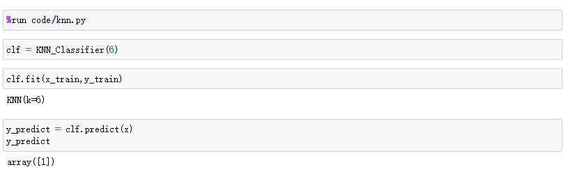
- 测试结果
KNN算法的优点
- 效果好
- 思想简单
- 对异常值不敏感。
- 需要的数学知识较少
- 直观完整的刻画机器学习应用的流程
KNN算法的缺点
- 计算复杂性高;空间复杂性高。
- 样本不平衡问题(即有些类别的样本数量很多,而其它样本的数量很少)
- 一般数值很大的时候不用这个,计算量太大。但是单个样本又不能太少,否则容易发生误分。
- 最大的缺点是无法给出数据的内在含义。